Population coding of time-varying sounds in the nonlemniscal inferior colliculus

Abstract

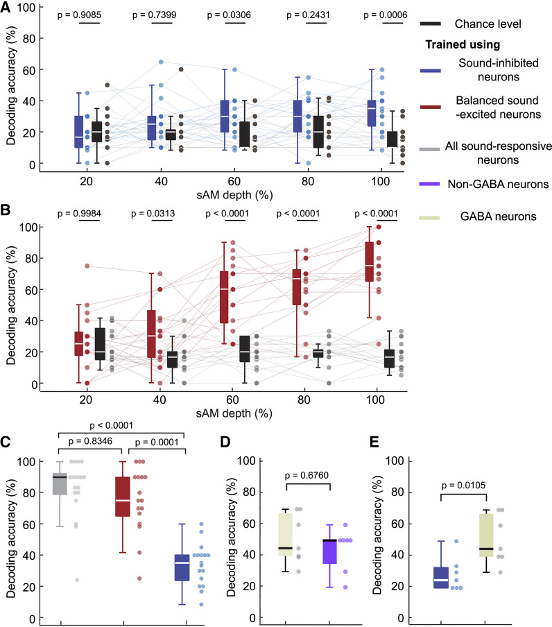
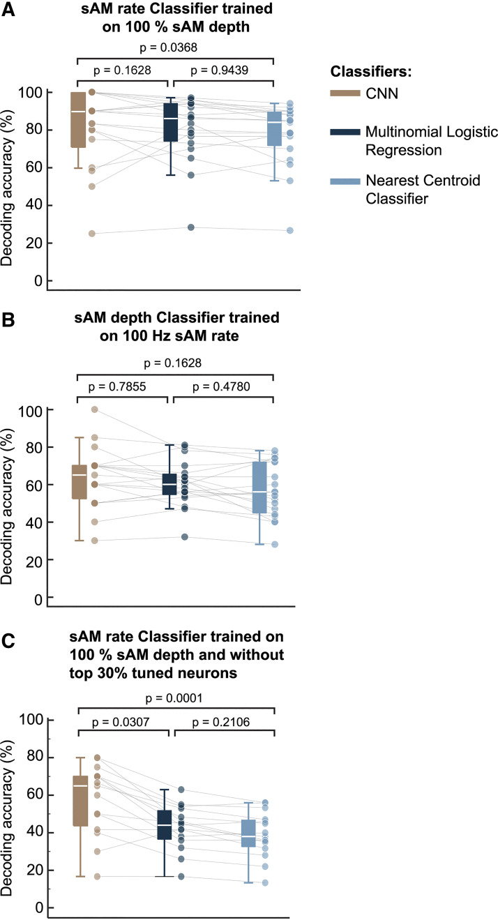
The inferior colliculus (IC) of the midbrain is important for complex sound processing, such as discriminating conspecific vocalizations and human speech. The IC's nonlemniscal, dorsal "shell" region is likely important for this process, as neurons in these layers project to higher-order thalamic nuclei that subsequently funnel acoustic signals to the amygdala and nonprimary auditory cortices, forebrain circuits important for vocalization coding in a variety of mammals, including humans. However, the extent to which shell IC neurons transmit acoustic features necessary to discern vocalizations is less clear, owing to the technical difficulty of recording from neurons in the IC's superficial layers via traditional approaches. Here, we use two-photon Ca²⁺ imaging in mice of either sex to test how shell IC neuron populations encode the rate and depth of amplitude modulation, important sound cues for speech perception. Most shell IC neurons were broadly tuned, with a low neurometric discrimination of amplitude modulation rate; only a subset was highly selective to specific modulation rates. Nevertheless, neural network classifier trained on fluorescence data from shell IC neuron populations accurately classified amplitude modulation rate, and decoding accuracy was only marginally reduced when highly tuned neurons were omitted from training data. Rather, classifier accuracy increased monotonically with the modulation depth of the training data, such that classifiers trained on full-depth modulated sounds had median decoding errors of ∼0.2 octaves. Thus, shell IC neurons may transmit time-varying signals via a population code, with perhaps limited reliance on the discriminative capacity of any individual neuron.NEW & NOTEWORTHY The IC's shell layers originate a "nonlemniscal" pathway important for perceiving vocalization sounds. However, prior studies suggest that individual shell IC neurons are broadly tuned and have high response thresholds, implying a limited reliability of efferent signals. Using Ca²⁺ imaging, we show that amplitude modulation is accurately represented in the population activity of shell IC neurons. Thus, downstream targets can read out sounds' temporal envelopes from distributed rate codes transmitted by populations of broadly tuned neurons.

Keywords: amplitude modulation; auditory system; calcium imaging; inferior colliculus.

Graphical abstract

Figure 1.

Responses of mouse shell IC neurons to sAM and unmodulated narrow-band noises. A: experimental setup of sound presentation and two-photon imaging of head-fixed, awake mice. B, left: an example of presented sAM narrow-band noises (100% sAM depth and 10 Hz sAM rate). Right: an example of presented unmodulated noises. C: example imaging FOV. D: example responses of sound-excited (left) and sound-inhibited (right) neurons to fully modulated sAM sounds. Data are means ± SE. E: proportion of sound-excited neurons in each imaging session. F: proportion of sound-excited neurons across different mice. Data are means ± SE. G: distribution of lifetime sparseness of sound-excited and sound-inhibited neurons. A neuron is maximally selective to sAM stimuli if its sparseness is 1 and is totally unselective if the sparseness is 0. Mann–Whitney U test. H: distribution of lifetime sparseness of sound-excited and sound-inhibited neurons from GCaMP6s and GCaMP6f datasets. P values reflect Šídák’s multiple comparisons following a two-way ANOVA, comparing the lifetime sparseness of sound-excited and -inhibited neurons recorded with GCaMP6f or GCaMP6s. Example of trial-averaged neuronal responses (left) and peak ΔF/F (right) of band pass (I), high pass (J), low pass (K), and band reject (L), broadly responsive (M) neurons under different sAM sounds. FOV, field of view; IC, inferior colliculus; sAM, sinusoidally amplitude modulated.

Figure 2.

sAM tuning of shell IC GABAergic and non-GABAergic neurons. A: tdTomato was expressed in GABAergic neurons in transgenic VGAT-ires-cre x Ai14 mice. B: example imaging FOV. C: proportion of GABAergic neurons in each imaging session (n = 13 imaging sessions in 4 mice). D: proportion of sound-excited GABAergic neurons in each imaging sessions. E: proportion of sound-excited GABAergic neurons across different animals. Data are means ± SE. F: distribution of tuning characteristics of non-GABAergic and GABAergic neurons. G: lifetime sparseness of GABAergic and non-GABAergic neurons. P values reflect Šídák’s multiple comparison between the lifetime sparseness of GABAergic and non-GABAergic neurons following a two-way ANOVA. FOV, field of view; IC, inferior colliculus; sAM, sinusoidally amplitude modulated.

Figure 3.

Neurometric sensitivity of individual shell IC neurons. A: schematic of neurometric sensitivity index (d-prime) analysis. Characteristic sAM rate is determined by the peak fluorescence response at different sAM rates (i). We binarize a neuron’s response as a hit if the mean neuronal response at its characteristic sAM rate exceeds three times the standard deviation of the baseline fluctuation on a single trial. Similarly, we count a false alarm response if a neuron’s average response at its noncharacteristic sAM rate exceeds three times the standard deviation of the baseline fluctuation (ii). The d-prime was then calculated for each neuron for all pairs of sAM depths for characteristic and other sAM rates (iii). B: distribution of d-prime at varying sAM depths for the characteristic sAM rate. Each line indicates a neuron displaying an increasing (pink) or decreasing (gray) trend across sAM depths for the characteristic sAM rate (see materials and methods). Data are means ± SD. Two-way ANOVA. Šídák’s multiple comparison between d-primes of sound-excited and sound-inhibited neurons. C, left: averaged d-prime of sound-excited neurons. Right: averaged d-prime of sound-inhibited neurons. D: trial-averaged fluorescence response to characteristic and noncharacteristic sAM rate. 689 neurons from 19 imaging sessions in 8 mice. Data are means ± SE. IC, inferior colliculus; sAM, sinusoidally amplitude modulated.

Figure 4.

Decoding sAM features using shell IC neural population activity. A: structure of the CNN classifier. A CNN classifier fed with Ca²⁺ signal time series was trained to classify sAM features. B: normalized confusion matrix of sAM depth and rate joint combination classification averaged across imaging sessions. C: normalized confusion matrix of sAM rate classification under a given sAM depth averaged across imaging sessions. D: decoding accuracy (n = 19 imaging sessions) of the sAM rate classifier under a given depth and the corresponding chance level. Two-way repeated-measures ANOVA. Šídák’s multiple comparison between the chance level accuracy and decoding accuracy trained using all neurons. E: one-vs.-rest ROC of sAM rate classification under 100% sAM depth. Data are means ± SD. F: d-prime of sAM rate classifier under 100% sAM depth. G: individual neuron d-prime distribution (under 100% sAM depth), with the corresponding highly sensitive neurons falling within top deciles (10%, 20%, 30% of d-prime). H: decoding accuracy (n = 15–16 imaging sessions) of the sAM rate classifier under 100% sAM depth, trained while excluding the top deciles (10%, 20%, and 30%) of neurons, selected based on their d-prime profiles in the left. To rectify the effect of the number of neurons on the decoding performance of the classifier, decoding accuracy of the classifier trained with a balanced number of randomly chosen neurons was visualized as control. Data are means ± SE and gray dots represent predictions from each imaging session. Two-way ANOVA. Šídák’s multiple comparison between the decoding accuracy trained without highly tuned neurons and the control. CNN, convolutional neural network; IC, inferior colliculus; ROC, receiver operating characteristic; sAM, sinusoidally amplitude modulated.

Figure 5.

Decoding sAM rate using sound-excited and sound-inhibited neurons. A: decoding accuracy (n = 17 imaging sessions) of sAM rate classifier trained using sound-inhibited neurons and corresponding chance level. Two-way repeated-measures ANOVA. Šídák’s multiple comparison between decoding accuracy trained using sound-inhibited and chance. B: decoding accuracy (n = 17 imaging sessions) of sAM rate classifier trained using sound-excited neurons and corresponding chance level. To ensure an equal number of sound-excited and sound-inhibited neurons, we randomly selected a subset of sound-excited neurons from each imaging session. Two-way repeated-measures ANOVA. Šídák’s multiple comparison between decoding accuracy trained using balanced sound-excited and chance. C: decoding accuracy (n = 17 imaging sessions) of sAM rate classifier trained using all sound-responsive, sound-excited, and sound-inhibited neurons under 100% sAM depth. Kruskal–Wallis test. Dunn’s multiple comparison between decoding accuracies trained under different conditions. D: decoding accuracy (n = 7 imaging sessions) of sAM rate classifier under 100% depth trained using balanced non-GABAergic neurons and GABAergic neurons. Mann–Whitney U test. E: decoding accuracy (n = 7 imaging sessions) of sAM rate classifier under 100% depth trained using balanced sound-inhibited neurons and GABAergic neurons. Mann–Whitney U test. sAM, sinusoidally amplitude modulated.

Figure 6.

Decoding sAM depth. A: decoding accuracy (n = 19 imaging sessions) of the sAM depth classifier under a given rate and its corresponding chance level. Two-way repeated-measures ANOVA. Šídák’s multiple comparison between decoding accuracy trained using all neurons and the chance. B: normalized confusion matrix of sAM depth classification under a given rate averaged across imaging sessions. sAM, sinusoidally amplitude modulated.

Figure 7.

Decoding sAM features using different classification models. A: decoding accuracy (n = 19 imaging sessions) of sAM rate classifier under 100% depth across three decoding models. B: decoding accuracy (n = 19 imaging sessions) of sAM depth classifier under 100 Hz rate across three decoding models. C: decoding accuracy (n = 15 imaging sessions) of sAM rate classifier under 100% depth, trained without top 30% tuned neurons. Friedman test for A, B, and C. Dunn’s multiple comparison between decoding accuracies trained using different decoding models. sAM, sinusoidally amplitude modulated.

Figure 8.

Representation of different sAM depths in the shell IC. A: for sAM rate classification, the decoder was trained using input data from a specific sAM depth. After training was complete, the decoder was evaluated on both original testing sets held back from training and extended testing sets (all datasets from other sAM depths). B: evaluation of the sAM rate classifier on extended testing sets (black) and held-back testing sets (red). n = 19 imaging session for each sAM depth. The curve was fitted using a Gaussian model. Friedman test for each subpanel. Dunn’s multiple comparison between decoding accuracies tested on held-back and extended testing sets. C: pattern correlation of each pair of sAM depths. Left: correlation of the trial-averaged neural population vector across two different sAM depths or rates on a per-frame basis. Data are means ± SE. Right: averaged correlation data during sound presentation. D: two-dimensional t-SNE map of shell IC neural population activity. Left: t-SNE map of neural population activity during baseline. Right: t-SNE map of neural population activity during sound presentation. E: t-SNE map of neural population data with a single sAM depth only. Each dot represents a single trial neural population activity. IC, inferior colliculus; sAM, sinusoidally amplitude modulated; t-SNE, t-distributed stochastic neighbor embedding.

Figure 9.

Binary classification of sAM and unmodulated sounds. A: binary classification paradigm: a CNN decoder was trained to classify sAM (with different sAM depths and rates) and unmodulated noise. B: decoding accuracy (n = 18 imaging sessions) of binary classification of sAM sounds and unmodulated noise and corresponding chance level. C: logistic curve fitting of the binary classification performance. Dashed lines, both horizontal and vertical, denotes the position of the half maximum on the fitted curve. D: pattern correlation between sAM sounds with different sAM depths and unmodulated sounds. For B and D, data are means ± SE. CNN, convolutional neural network; sAM, sinusoidally amplitude modulated.

Figure 10.

Neuronal responses to narrowly spaced sAM rates in the shell IC. A: examples of modulation transfer functions to fully modulated sAM sounds with 30–150 Hz sAM rates. Top: peak response of example neurons at varying sAM rates and 100% sAM depth. Bottom: trial-averaged fluorescence traces of example neurons. B: distribution of d-prime of shell IC neurons (520 neurons from 9 imaging sessions in 5 mice). C: t-SNE map of shell IC population responses to narrowly spaced sAM rates. Each dot represents neural population activity in a single trial. D: regression performance (n = 9 imaging sessions) of CNN decoder using population fluorescence data of shell IC neurons with narrowly spaced sAM rates and 100% sAM depth. Each dot is the prediction of a single trial in testing sets. The coordinates are plotted on a logarithmic scale of base 10. E: distribution of decoding errors in octaves. F: example imaging FOV. Trial-averaged responses (G) and peak of response (H) of two example neurons to sAM sounds with 16 kHz and 8 kHz center frequencies for the noise carrier. I: sAM rate decoding performance: sAM rate decoder was trained using data from sAM sounds with central frequency of either 8 kHz or 16 kHz for the noise carrier. After training, the decoder was evaluated on both original held-back testing sets with the same center frequency as in the training set, and extended testing sets with a different central frequency of the carrier. J and K: distribution of decoding error in octave (n = 3 imaging sessions for each carrier). Wilcoxon signed-rank test. FOV, field of view; IC, inferior colliculus; sAM, sinusoidally amplitude modulated.

References

1. Drullman R, Festen JM, Plomp R. Effect of temporal envelope smearing on speech reception. J Acoust Soc Am 95: 2670–2680, 1994. doi:10.1121/1.409836. - DOI - PubMed
1. Elliott TM, Theunissen FE. The modulation transfer function for speech intelligibility. PloS Comput Biol 5: e1000302, 2009. doi:10.1371/journal.pcbi.1000302. - DOI - PMC - PubMed
1. Gallun F, Souza P. Exploring the role of the modulation spectrum in phoneme recognition. Ear Hear 29: 800–813, 2008. doi:10.1097/AUD.0b013e31817e73ef. - DOI - PMC - PubMed
1. Koumura T, Terashima H, Furukawa S. Cascaded tuning to amplitude modulation for natural sound recognition. J Neurosci 39: 5517–5533, 2019. doi:10.1523/JNEUROSCI.2914-18.2019. - DOI - PMC - PubMed
1. Koumura T, Terashima H, Furukawa S. Human-like modulation sensitivity emerging through optimization to natural sound recognition. J Neurosci 43: 3876–3894, 2023. doi:10.1523/JNEUROSCI.2002-22.2023. - DOI - PMC - PubMed
Publication types
LinkOut - more resources