Lusca: FIJI (ImageJ) based tool for automated morphological analysis of cellular and subcellular structures

Abstract

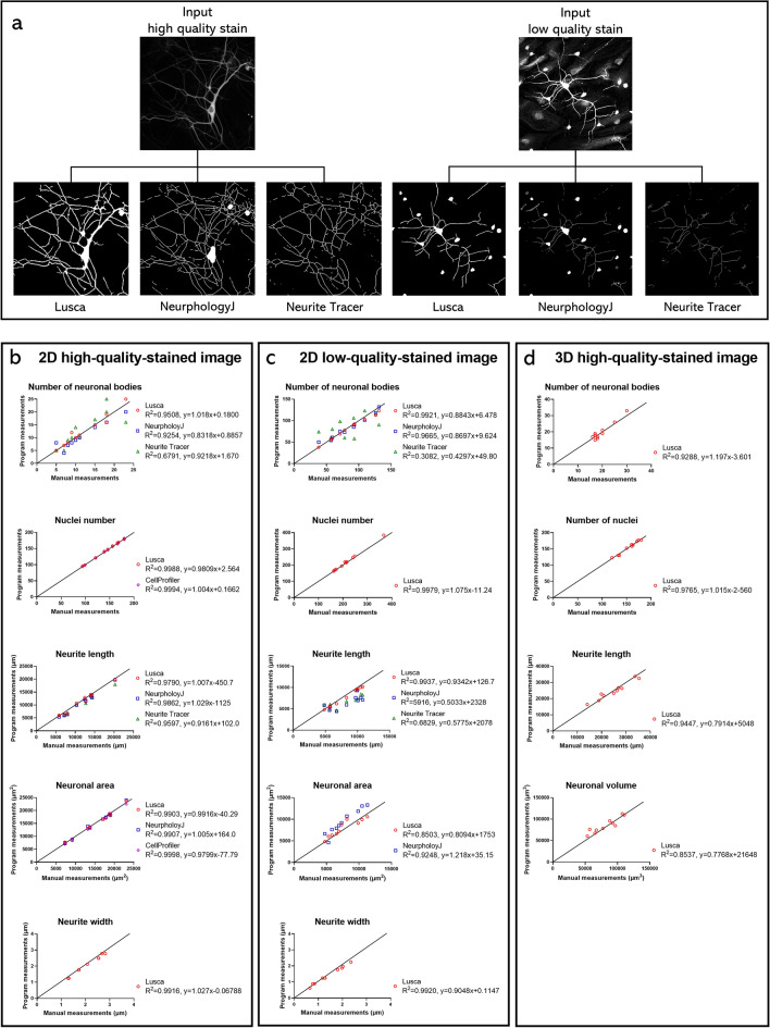
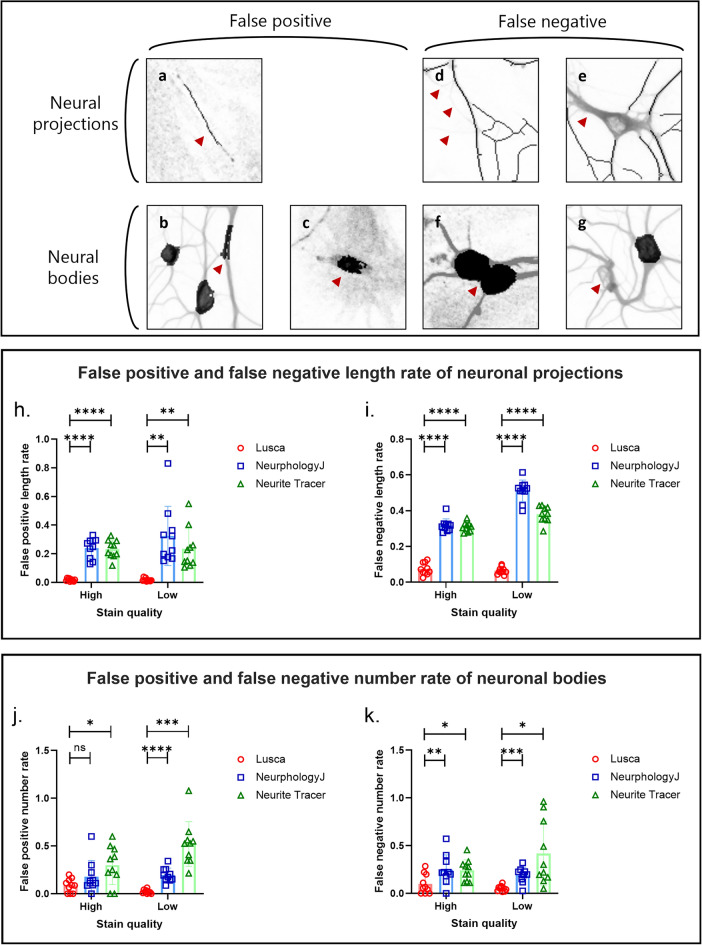
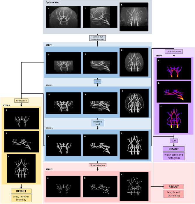
The human body consists of diverse subcellular, cellular and supracellular structures. Neurons possess varying-sized projections that interact with different cellular structures leading to the development of highly complex morphologies. Aiming to enhance image analysis of complex biological forms including neurons using available FIJI (ImageJ) plugins, Lusca, an advanced open-source tool, was developed. Lusca utilizes machine learning for image segmentation with intensity and size thresholds. It performs particle analysis to ascertain parameters such as area/volume, quantity, and intensity, in addition to skeletonization for determining length, branching, and width. Moreover, in conjunction with colocalization measurements, it provides an extensive set of 29 morphometric parameters for both 2D and 3D analysis. This is a significant enhancement compared to other scripts that offer only 5-15 parameters. Consequently, it ensures quicker and more precise quantification by effectively eliminating noise and discerning subtle details. With three times larger execution speed, fewer false positive and negative results, and the capacity to measure various parameters, Lusca surpasses other existing open-source solutions. Its implementation of machine learning-based segmentation facilitates versatile applications for different cell types and biological structures, including mitochondria, fibres, and vessels. Lusca's automated and precise measurement capability makes it an ideal choice for diverse biological image analyses.

Figure 1

Pipeline for image analysis of neural projections and bodies. Blue squares represent image segmentation, while grey, orange, green, red, violet, and yellow represent different options for image analysis. These include colocalization, neural bodies, neural projections, length and branching, width, and area, number, and intensity, respectively. Step 1 shows the enlarged input images of neurons and nuclei stained with MAP2 (red), SMI312 (green), and DAPI (cyan). ROIs are segmented from the background with TWS in step 2, following intensity, area, and circularity thresholding to obtain the segmented image in step 3. “Neural bodies” analysis includes the calculation of area, number, and intensity for both nuclei and soma images. Neural bodies image is acquired by using the Boolean operator “AND” on previously dilated nuclei image and neuron image from step 3 to avoid false signals. The area, number, and intensity of both neural bodies and nuclei are calculated with the particle analyser after redirection to the corresponding input images (orange square, step 4). Analysis option “Neural projections” includes the calculation of area, number, intensity, length, branching, and width. Particle analysis was performed again to obtain area, number, and intensity results (green square, step 4). Length and branching are calculated after forming skeletons in step 5, while width calculation further involves the transformation of the step 5 image into a 32-bit image. Following thresholding and deduction of 255, values of NaN for the background pixels, and 0 for skeletons, are obtained. Simultaneously, using the Local Thickness on the image from step 3, accurate width dimensions are achieved (step 6). The images from step 5 and step 6 are added to obtain the image in step 7 from which width results are calculated. The separation of these options into distinct squares (red, violet, and yellow) facilitates better user comprehension and easier application, especially considering the versatility of Lusca in analysing various biological objects beyond neurons.

Figure 2

Qualitative and quantitative comparison of different scripts for neuron analysis with Lusca and manual tracing on 2D high and low-quality-stained and 3D images. Comparison between open-source programs, Lusca, and manual tracing performed on MAP2 high and low-quality-stained input images. (a) Qualitative comparison of Lusca, NeurphologyJ, and Neurite Tracer final output images for each image stain quality. Datasets (neuronal bodies and nuclear count, neurite length and width, and neuron area/volume) generated by each open-source program, Lusca and manual measurements subjected to linear regression for 2D (b) high and (c) low-quality-stained images, as well as (d) 3D images. The equations for the lines of best fit and the coefficients of determination are presented in the figure key.

Figure 3

False positive and negative operational classifications and measurements rate comparison between NeurphologyJ, NeuriteTracer and Lusca. False negative signal defined as an unrecognized visible signal by the macro. False positive signal characterised by the macro but lacking an actual signal. Recognised false positive signals for neural projections: (a) background noise mistaken for neurite, while for neural bodies these include (b) thick neurite and (c) background noise misplaced for neural body. False negative signals for neural projections: (d) neurites recognised as background and (e) thick neurite misplaced to neural bodies, and for neural bodies (f) two connected neural bodies and (g) neural body recognised as background. For further comparison of ImageJ/FIJI macros, false positive and negative signals measured for each script on high and low-quality-stained MAP2 neuron images: false positive neurite length rate (h), false negative neurite length rate (i), false positive count rate of neuronal bodies (j), false negative count rate of neuronal bodies (k).

Figure 4

Lusca pipeline applied for morphological 3D magnetic resonance angiography (MRA) stack analysis. For 3D perception the anatomical planes (a) coronal, (b) sagittal and (c) transversal are shown. Blue, yellow, red, and violet squares represent image segmentation, area, number and intensity, length and branching, and width measurements respectively. The anatomical landmarks of MRA stacks used to standardize the volume and position of the maximum intensity projection ROIs (Optional step, grey square). Vessels on the input images in step 1 segmented from the background with TWS in step 2 and, after area and intensity thresholding, the step 3 segmented image is acquired. In step 4, after redirection of segmented image to the input image, the area, number, and intensity are obtained. For length and branching measurements, in step 3 the image undergoes skeletonization and analysis. Width is calculated by applying Local thickness mask on the image from step 3 to get step 6 image. Simultaneously, the threshold is applied to the 32-bit image from step 5, and after subtracting 255 values NaN for the background and 0 for skeleton pixels are obtained. Images from steps 5 and 6 are added to get step 7 image that serves for width calculations.

Figure 5

Lusca pipeline for morphological analysis of mitochondria. Blue, red, and yellow squares represent image segmentation, length and branching, and area, count and intensity measurements respectively. Mitochondria immunocytochemistry images in (a) normoxic and (b) after oxygen–glucose deprivation treatment were stained with Tomm20 antibody. Mitochondria (step 1) are segmented from the background with TWS in step 2 and after area, intensity and circularity thresholding, the step 3 image is acquired. In step 4 after redirecting the input image the result area, count and intensity are obtained. For further length and branching measurements, the step 3 image is skeletonized and analysed (step 5).

References

1. Titus ADJ, et al. Hypobaric hypoxia-induced dendritic atrophy of hippocampal neurons is associated with cognitive impairment in adult rats. Neuroscience. 2007;145:265–278. doi: 10.1016/j.neuroscience.2006.11.037. - DOI - PubMed
1. York, E. M., LeDue, J. M., Bernier, L.-P. & MacVicar, B. A. 3DMorph automatic analysis of microglial morphology in three dimensions from ex vivo and in vivo imaging. eNeuro5(6), ENEURO.0266–18.2018. (2018). - PMC - PubMed
1. Abramoff MD, Magalhaes PJ, Ram SJ. Image processing with ImageJ. Biophoton. Int. 2004;11:36–42.
1. Carpenter AE, et al. Cell Profiler: Image analysis software for identifying and quantifying cell phenotypes. Genome Biol. 2006;7:R100. doi: 10.1186/gb-2006-7-10-r100. - DOI - PMC - PubMed
1. Meijering E, et al. Design and validation of a tool for neurite tracing and analysis in fluorescence microscopy images. Cytometry. A. 2004;58:167–176. doi: 10.1002/cyto.a.20022. - DOI - PubMed