Temporal Supervised Contrastive Learning for Modeling Patient Risk Progression

Abstract

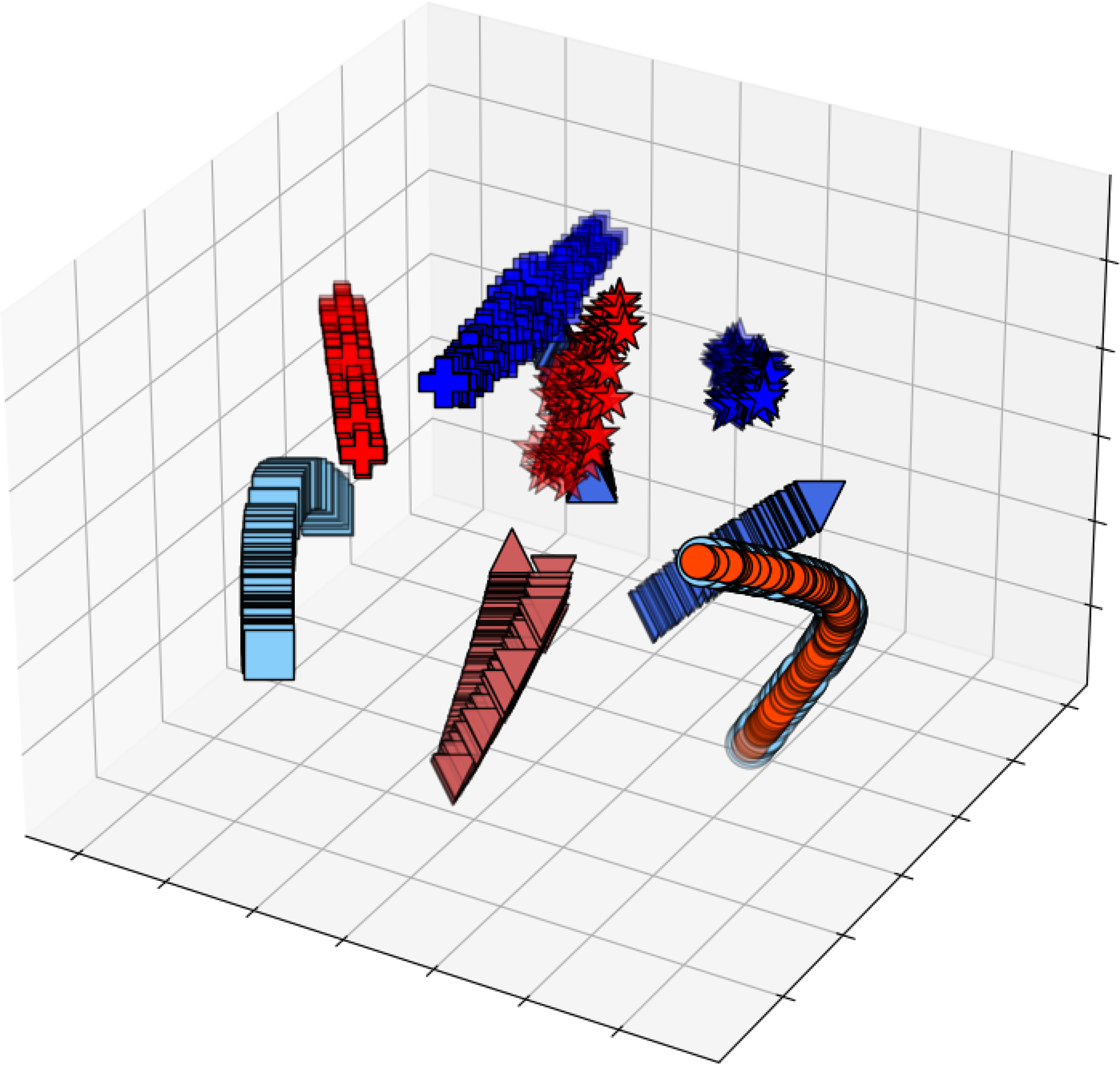
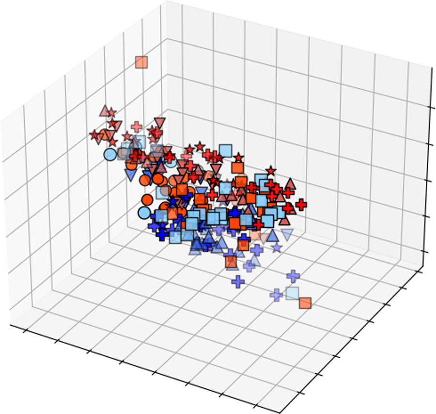
We consider the problem of predicting how the likelihood of an outcome of interest for a patient changes over time as we observe more of the patient's data. To solve this problem, we propose a supervised contrastive learning framework that learns an embedding representation for each time step of a patient time series. Our framework learns the embedding space to have the following properties: (1) nearby points in the embedding space have similar predicted class probabilities, (2) adjacent time steps of the same time series map to nearby points in the embedding space, and (3) time steps with very different raw feature vectors map to far apart regions of the embedding space. To achieve property (3), we employ a nearest neighbor pairing mechanism in the raw feature space. This mechanism also serves as an alternative to "data augmentation", a key ingredient of contrastive learning, which lacks a standard procedure that is adequately realistic for clinical tabular data, to our knowledge. We demonstrate that our approach outperforms state-of-the-art baselines in predicting mortality of septic patients (MIMIC-III dataset) and tracking progression of cognitive impairment (ADNI dataset). Our method also consistently recovers the correct synthetic dataset embedding structure across experiments, a feat not achieved by baselines. Our ablation experiments show the pivotal role of our nearest neighbor pairing.

Keywords: contrastive learning; nearest neighbors; time series analysis.

Figure A.1:

Setup for MIMIC Experiments at Inference time from Temporal-SCL: First, we extract time series data for each patient from a time window around their sepsis onset within their complete ICU data timeline. This time series data is transformed into multiple time steps at 4-hour intervals. The resulting time series will have its features at each time step mapped onto the embedding space learned by our encoder. Finally, these resulting embeddings will be passed through our predictor network to predict the ICU mortality of each patient at every time step.

Figure A.2:

Setup for ADNI Experiment at Inference time from Temporal-SCL: First, we extract time series data for each patient from their complete timeline of available data spanning all the 6-month follow-up visits. This time series data maintains the same 6-month interval time steps as the raw data, with each time step having its own true class label representing one of the three possible brain function states. The resulting time series will have its features at each time step mapped onto the embedding space learned by our encoder. Subsequently, these resulting embeddings will be passed through our predictor network to predict the brain function class of each patient at every time step.

Figure A.3:

Embedding space representation of the test trajectories of simulated dataset. For (a)-(j) 3D Embedding Space of baselines are shown which includes the purely supervised methods ((a)-(d)), predictive clustering methods ((e), (f)), and self-supervised learning methods ((g)-(j)). In (f)-(i), Hyperspherical Embedding of various ablated versions of Temporal-SCL is shown.

Figure A.3:

Embedding space representation of the test trajectories of simulated dataset. For (a)-(j) 3D Embedding Space of baselines are shown which includes the purely supervised methods ((a)-(d)), predictive clustering methods ((e), (f)), and self-supervised learning methods ((g)-(j)). In (f)-(i), Hyperspherical Embedding of various ablated versions of Temporal-SCL is shown.

Figure A.3:

Embedding space representation of the test trajectories of simulated dataset. For (a)-(j) 3D Embedding Space of baselines are shown which includes the purely supervised methods ((a)-(d)), predictive clustering methods ((e), (f)), and self-supervised learning methods ((g)-(j)). In (f)-(i), Hyperspherical Embedding of various ablated versions of Temporal-SCL is shown.

Figure A.3:

Embedding space representation of the test trajectories of simulated dataset. For (a)-(j) 3D Embedding Space of baselines are shown which includes the purely supervised methods ((a)-(d)), predictive clustering methods ((e), (f)), and self-supervised learning methods ((g)-(j)). In (f)-(i), Hyperspherical Embedding of various ablated versions of Temporal-SCL is shown.

Figure A.3:

Embedding space representation of the test trajectories of simulated dataset. For (a)-(j) 3D Embedding Space of baselines are shown which includes the purely supervised methods ((a)-(d)), predictive clustering methods ((e), (f)), and self-supervised learning methods ((g)-(j)). In (f)-(i), Hyperspherical Embedding of various ablated versions of Temporal-SCL is shown.

Figure A.3:

Embedding space representation of the test trajectories of simulated dataset. For (a)-(j) 3D Embedding Space of baselines are shown which includes the purely supervised methods ((a)-(d)), predictive clustering methods ((e), (f)), and self-supervised learning methods ((g)-(j)). In (f)-(i), Hyperspherical Embedding of various ablated versions of Temporal-SCL is shown.

Figure A.3:

Embedding space representation of the test trajectories of simulated dataset. For (a)-(j) 3D Embedding Space of baselines are shown which includes the purely supervised methods ((a)-(d)), predictive clustering methods ((e), (f)), and self-supervised learning methods ((g)-(j)). In (f)-(i), Hyperspherical Embedding of various ablated versions of Temporal-SCL is shown.

Figure A.3:

Embedding space representation of the test trajectories of simulated dataset. For (a)-(j) 3D Embedding Space of baselines are shown which includes the purely supervised methods ((a)-(d)), predictive clustering methods ((e), (f)), and self-supervised learning methods ((g)-(j)). In (f)-(i), Hyperspherical Embedding of various ablated versions of Temporal-SCL is shown.

Figure A.3:

Embedding space representation of the test trajectories of simulated dataset. For (a)-(j) 3D Embedding Space of baselines are shown which includes the purely supervised methods ((a)-(d)), predictive clustering methods ((e), (f)), and self-supervised learning methods ((g)-(j)). In (f)-(i), Hyperspherical Embedding of various ablated versions of Temporal-SCL is shown.

Figure A.3:

Embedding space representation of the test trajectories of simulated dataset. For (a)-(j) 3D Embedding Space of baselines are shown which includes the purely supervised methods ((a)-(d)), predictive clustering methods ((e), (f)), and self-supervised learning methods ((g)-(j)). In (f)-(i), Hyperspherical Embedding of various ablated versions of Temporal-SCL is shown.

Figure A.3:

Embedding space representation of the test trajectories of simulated dataset. For (a)-(j) 3D Embedding Space of baselines are shown which includes the purely supervised methods ((a)-(d)), predictive clustering methods ((e), (f)), and self-supervised learning methods ((g)-(j)). In (f)-(i), Hyperspherical Embedding of various ablated versions of Temporal-SCL is shown.

Figure A.3:

Embedding space representation of the test trajectories of simulated dataset. For (a)-(j) 3D Embedding Space of baselines are shown which includes the purely supervised methods ((a)-(d)), predictive clustering methods ((e), (f)), and self-supervised learning methods ((g)-(j)). In (f)-(i), Hyperspherical Embedding of various ablated versions of Temporal-SCL is shown.

Figure A.3:

Embedding space representation of the test trajectories of simulated dataset. For (a)-(j) 3D Embedding Space of baselines are shown which includes the purely supervised methods ((a)-(d)), predictive clustering methods ((e), (f)), and self-supervised learning methods ((g)-(j)). In (f)-(i), Hyperspherical Embedding of various ablated versions of Temporal-SCL is shown.

Figure A.3:

Embedding space representation of the test trajectories of simulated dataset. For (a)-(j) 3D Embedding Space of baselines are shown which includes the purely supervised methods ((a)-(d)), predictive clustering methods ((e), (f)), and self-supervised learning methods ((g)-(j)). In (f)-(i), Hyperspherical Embedding of various ablated versions of Temporal-SCL is shown.

Figure A.4:

Heatmap showing how features (rows) vary across clusters (columns) for the sepsis cohort of the MIMIC dataset when using clustering on Temporal-SCL learned embedding space. Heatmap intensity values can be thought of as the conditional probability of seeing a feature value (row) conditioned on being in a cluster (column); these probabilities are estimated using test set snapshots. Columns are ordered left to right in increasing fraction of test set snapshots that come from a time series that has a final outcome of death.

Figure A.5:

Heatmap showing how features (rows) vary across clusters (columns) for the ADNI dataset when using clustering on Temporal-SCL learned embedding space. Heatmap intensity values can be thought of as the conditional probability of seeing a feature value (row) conditioned on being in a cluster (column); these probabilities are estimated using test set snapshots. Columns are ordered left to right in increasing fraction of test set snapshots that come from a time series that has a final outcome of Alzheimer’s Disease.

Figure A.6:

Heatmap showing how features (rows) vary across clusters (columns) for the MIMIC dataset when using clustering on the Raw features instead of model embeddings. Heatmap intensity values can be thought of as the conditional probability of seeing a feature value (row) conditioned on being in a cluster (column); these probabilities are estimated using test set snapshots. Columns are ordered left to right in increasing fraction of test set snapshots that come from a time series that has a final outcome of death.

Figure 3.1:

Overview of Temporal-SCL amounts to standard neural net classifier training with cross-entropy loss, we omit further details.

Figure 3.1:

Overview of Temporal-SCL amounts to standard neural net classifier training with cross-entropy loss, we omit further details.

Figure 3.1:

Overview of Temporal-SCL amounts to standard neural net classifier training with cross-entropy loss, we omit further details.

Figure 3.2:

Heatmap showing how features (rows) vary across clusters (columns) for the sepsis cohort of the MIMIC dataset. Heatmap intensity values can be thought of as the conditional probability of seeing a feature value (row) conditioned on being in a cluster (column); these probabilities are estimated using test set snapshots. Columns are ordered left to right in increasing fraction of test set snapshots that come from a time series that has a final outcome of death.

Figure 4.1:

Synthetic dataset: panel (a) shows the only 4 possible time series trajectories (each true embedding vector state has a unique color-shape combination; there are 10 such states); every time series has 3 time steps and belongs to one of two classes red/blue. Panels (b)-(e) show learned embedding spaces of four methods; only Temporal-SCL correctly recovers the 10 ground truth states. A version of this figure with embeddings of all methods evaluated is in Fig. A.3.

Figure 4.1:

Synthetic dataset: panel (a) shows the only 4 possible time series trajectories (each true embedding vector state has a unique color-shape combination; there are 10 such states); every time series has 3 time steps and belongs to one of two classes red/blue. Panels (b)-(e) show learned embedding spaces of four methods; only Temporal-SCL correctly recovers the 10 ground truth states. A version of this figure with embeddings of all methods evaluated is in Fig. A.3.

Figure 4.1:

Synthetic dataset: panel (a) shows the only 4 possible time series trajectories (each true embedding vector state has a unique color-shape combination; there are 10 such states); every time series has 3 time steps and belongs to one of two classes red/blue. Panels (b)-(e) show learned embedding spaces of four methods; only Temporal-SCL correctly recovers the 10 ground truth states. A version of this figure with embeddings of all methods evaluated is in Fig. A.3.

Figure 4.1:

Synthetic dataset: panel (a) shows the only 4 possible time series trajectories (each true embedding vector state has a unique color-shape combination; there are 10 such states); every time series has 3 time steps and belongs to one of two classes red/blue. Panels (b)-(e) show learned embedding spaces of four methods; only Temporal-SCL correctly recovers the 10 ground truth states. A version of this figure with embeddings of all methods evaluated is in Fig. A.3.

Figure 4.1:

Synthetic dataset: panel (a) shows the only 4 possible time series trajectories (each true embedding vector state has a unique color-shape combination; there are 10 such states); every time series has 3 time steps and belongs to one of two classes red/blue. Panels (b)-(e) show learned embedding spaces of four methods; only Temporal-SCL correctly recovers the 10 ground truth states. A version of this figure with embeddings of all methods evaluated is in Fig. A.3.

References

1. Aguiar Henrique, Santos Mauro, Watkinson Peter, and Zhu Tingting. Learning of cluster-based feature importance for electronic health record time-series. In International Conference on Machine Learning, 2022.
1. Bardes Adrien, Ponce Jean, and LeCun Yann. Vicreg: Variance-invariance-covariance regularization for self-supervised learning. arXiv preprint arXiv:2105.04906, 2021.
1. Carr Oliver, Javer Avelino, Rockenschaub Patrick, Parsons Owen, and Durichen Robert. Longitudinal patient stratification of electronic health records with flexible adjustment for clinical outcomes. In Machine Learning for Health, 2021.
1. Chen Ting, Kornblith Simon, Norouzi Mohammad, and Hinton Geoffrey. A simple framework for contrastive learning of visual representations. In International Conference on Machine Learning, 2020.
1. Choi Edward, Bahadori Mohammad Taha, Sun Jimeng, Kulas Joshua, Schuetz Andy, and Stewart Walter. RETAIN: An interpretable predictive model for healthcare using reverse time attention mechanism. In Advances in Neural Information Processing Systems, 2016.
LinkOut - more resources