SpatialcoGCN: deconvolution and spatial information-aware simulation of spatial transcriptomics data via deep graph co-embedding

Abstract

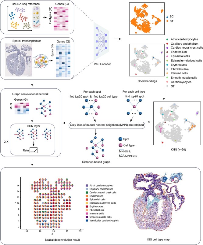
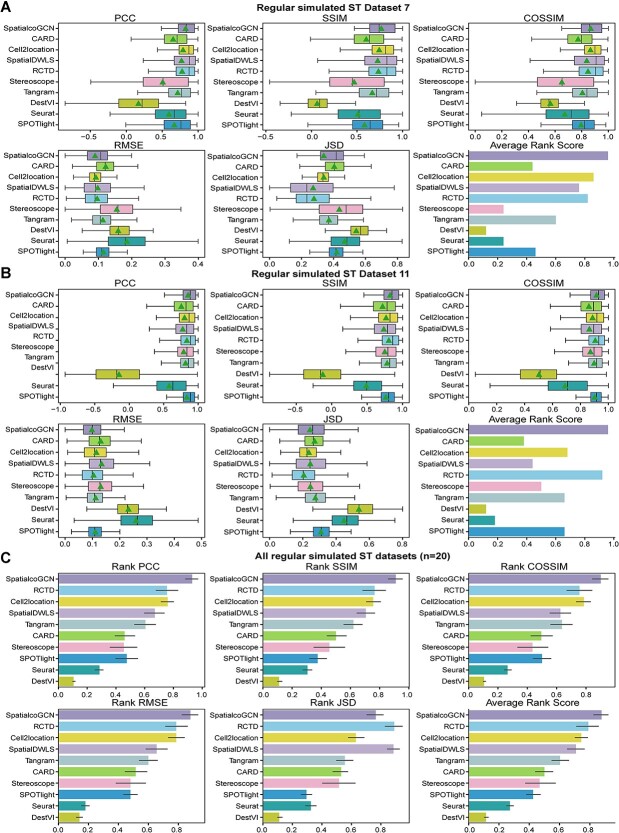
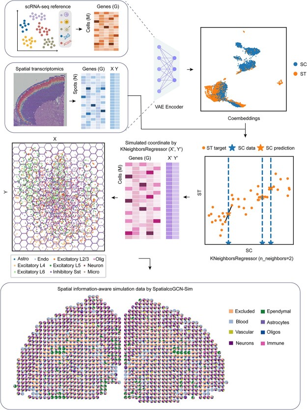
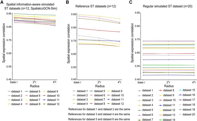
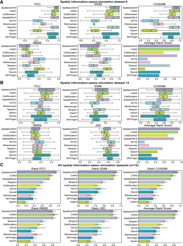
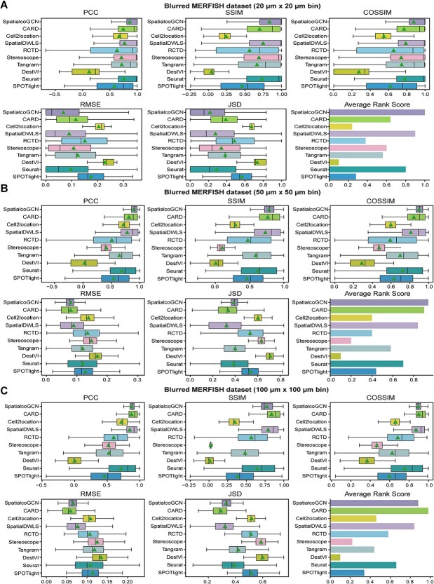
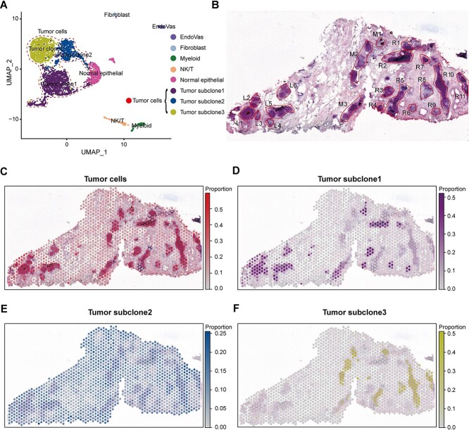
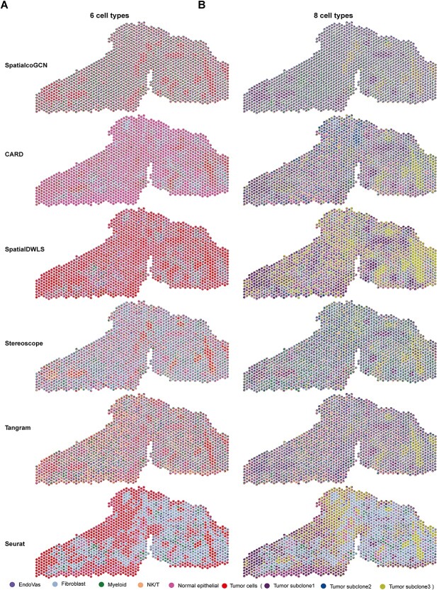
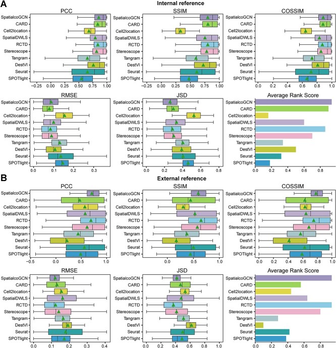
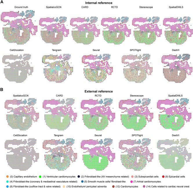
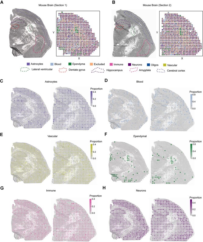
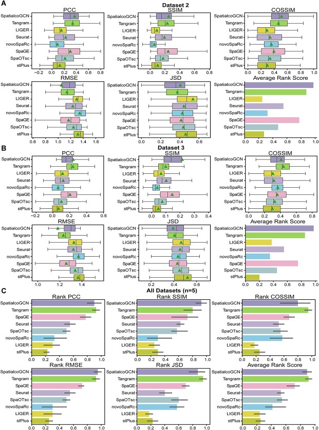
Spatial transcriptomics (ST) data have emerged as a pivotal approach to comprehending the function and interplay of cells within intricate tissues. Nonetheless, analyses of ST data are restricted by the low spatial resolution and limited number of ribonucleic acid transcripts that can be detected with several popular ST techniques. In this study, we propose that both of the above issues can be significantly improved by introducing a deep graph co-embedding framework. First, we establish a self-supervised, co-graph convolution network-based deep learning model termed SpatialcoGCN, which leverages single-cell data to deconvolve the cell mixtures in spatial data. Evaluations of SpatialcoGCN on a series of simulated ST data and real ST datasets from human ductal carcinoma in situ, developing human heart and mouse brain suggest that SpatialcoGCN could outperform other state-of-the-art cell type deconvolution methods in estimating per-spot cell composition. Moreover, with competitive accuracy, SpatialcoGCN could also recover the spatial distribution of transcripts that are not detected by raw ST data. With a similar co-embedding framework, we further established a spatial information-aware ST data simulation method, SpatialcoGCN-Sim. SpatialcoGCN-Sim could generate simulated ST data with high similarity to real datasets. Together, our approaches provide efficient tools for studying the spatial organization of heterogeneous cells within complex tissues.

Keywords: cell type deconvolution; graph-based deep learning; spatial transcriptomics; spatial transcriptomics data simulation.

Figure 1

Schematic overview of SpatialcoGCN, an ST data deconvolution method. SpatialcoGCN first transformed scRNA-seq data by summing the expression profiles of cells of the same cell type. The transformed scRNA-seq data and ST data were then projected into a shared embedding space via the encoder architecture of VAE. In this low-dimensional embedding space, SpatialcoGCN established a link graph between cells and spots based on KNN distances. The link graph was merged from spot-to-spot and spot-to-cell subgraphs, and only connections passed the mutual nearest neighbor criterion were retained. Taking the link graph, and the original expression matrix of cell types/spots as the input, a GCN to propagate both transformed scRNA-seq and ST data into the latent layer and solve the mapping matrix that estimate the compositions of different cell types for each spot. Consequently, the compositions of cells in ST data can be accurately learned and predicted.

Figure 2

Evaluation of deconvolution performance on regular simulated ST datasets. Comparing the performance of SpatialcoGCN against nine other methods with the capability of deconvoluting cell types for each ST spot, we present our results as boxplots and bar plots. Boxplots: center line, median; box limits, upper and lower quartiles; triangle: mean. Bar plots: data are presented as mean values ± 90% confidence intervals. (A) The boxplots of PCC, SSIM, COSSIM, RMSE, and JSD, as well as the bar plot of ARS (aggregated from PCC, SSIM, COSSIM, RMSE, and JSD; see Methods) illustrating the cell-type composition prediction performance on the regular simulated ST dataset 7. (B) PCC, SSIM, COSSIM, RMSE and JSD, as well as the bar plot of ARS illustrating the cell-type composition prediction performance on the regular simulated ST dataset 11. (C) The bar plots of Rank PCC, Rank SSIM, Rank COSSIM, Rank RMSE, Rank JSD and ARS summarizing the performance on all of the 20 regular simulated ST datasets.

Figure 3

Schematic overview of SpatialcoGCN-Sim, a spatial information-aware ST data simulation method. First, the scRNA-seq data and ST data were projected into a co-embedding space with the aid of the VAE. Subsequently, KNeighborsRegressor was applied in the low-dimensional embedding space to predict the 2D coordinates of the cell based on the coordinates of the spots. To reduce the noise, hexagonal grid representation was employed to represent low-spatial-resolution spots and the center of the hexagon was selected as the coordinates of the spots. Finally, the spatial information–aware simulation data were generated by averaging and normalizing the gene expression of each spot.

Figure 4

Comparison of spatial expression correlation of different simulated ST datasets and real ST datasets. (A) The spatial expression correlation of 12 spatial information-aware simulated ST datasets generated by SpatialcoGCN-Sim. (B) The spatial expression correlation of 12 reference ST datasets. (C) The spatial expression correlation of 20 regular simulated ST datasets.

Figure 5

Evaluation of deconvolution performance on spatial information–aware simulated datasets. Comparing the performance of SpatialcoGCN against nine other methods with the capability of deconvoluting cell types for each ST spot, we present our results as boxplots and bar plots. Boxplots: center line, median; box limits, upper and lower quartiles; triangle: mean. Bar plots: data are presented as mean values ± 90% confidence intervals. (A) The boxplots of PCC, SSIM, COSSIM, RMSE and JSD, as well as the bar plot of ARS (aggregated from PCC, SSIM, COSSIM, RMSE and JSD; see Methods) illustrating the cell type composition prediction performance on the spatial information–aware simulated ST dataset 8. (B) PCC, SSIM, COSSIM, RMSE and JSD, as well as the bar plot of ARS illustrating the cell-type composition prediction performance on the spatial information–aware simulated ST dataset 12. (C) The bar plots of Rank PCC, Rank SSIM, Rank COSSIM, Rank RMSE, Rank JSD and ARS summarizing the performance on all of the 12 spatial information–aware simulated ST datasets.

Figure 6

Evaluation of deconvolution performance in the blurred MERFISH datasets at different resolutions. Comparing the performance of SpatialcoGCN against nine other methods with the capability of deconvoluting cell types for each ST spot, we present our results as boxplots and bar plots. Boxplots: center line, median; box limits, upper and lower quartiles; triangle: mean. Bar plots: data are presented as mean values ± 90% confidence intervals. (A) The boxplots of PCC, SSIM, COSSIM, RMSE and JSD, along with the bar plot for ARS (aggregated from PCC, SSIM, COSSIM, RMSE and JSD, see Methods) illustrating the cell-type composition prediction performance on the blurred MERFISH dataset at 20 μm resolution (i.e. blurred with 20 μm × 20 μm bin, see Methods). (B) The boxplots of PCC, SSIM, COSSIM, RMSE and JSD, along with the bar plot for ARS illustrating the cell-type composition prediction performance on the blurred MERFISH dataset at 50 μm resolution. (C) The boxplots of PCC, SSIM, COSSIM, RMSE and JSD, along with the bar plot for ARS illustrating the cell-type composition prediction performance on the blurred MERFISH dataset at 100 μm resolution.

Figure 7

Visualization of SpatialcoGCN’s deconvolution results on DCIS datasets. (A) UMAP of DCIS scRNA-seq reference, showing the six (five non-tumor cell types plus one tumor cell) or the eight (five non-tumor cell types plus three tumor subclones) cell type categorization. (B) H&E image of the DCIS tissue section with annotated ductal tumor regions. (C) The spatial distribution of tumor cells estimated by SpatialcoGCN. (D) The spatial distribution of tumor subclone1 estimated by SpatialcoGCN. (E) The spatial distribution of tumor subclone2 estimated by SpatialcoGCN. (F) The spatial distribution of tumor subclone3 estimated by SpatialcoGCN.

Figure 8

Comparison of deconvolution results by different methods on DCIS datasets. The spatial distributions of cell type proportion predicted by SpatialcoGCN and other five deconvolution methods using (A) six cell types scRNA-seq reference and (B) eight cell types scRNA-seq reference, respectively, are shown. Each pie represents the cell type proportions in each spot in the ST slide, and colors represent different cell types.

Figure 9

Performance of SpatialcoGCN on developing human heart ISS data. The boxplots of PCC, SSIM, COSSIM, RMSE and JSD, along with the bar plot for ARS illustrating the cell type composition prediction performance on the developing human heart ISS data using the (A) internal reference and (B) external reference, are shown.

Figure 10

Visualization of SpatialcoGCN’s deconvolution results on developing human heart ISS data. The spatial distributions of cell type proportion estimated for developing human-heart-tissue ISS data using (A) internal reference and (B) external reference, are shown.

Figure 11

Deconvolution result of SpatialcoGCN on the mouse brain dataset. (A, B) Spatial scatter pie plot representing the proportions of the cells from the reference atlas within the two captured sections in the adult mouse brain. Two different sections used are: ST1 (ST array, 100 μm spots) and ST2 (ST array, 100 μm spots). The matched histological images are shown, on which the featured brain regions are annotated. (C–H) The spatial distributions of cell type proportion predicted by SpatialcoGCN for each cell type and on each section.

Figure 12

Evaluation of the performance of SpatialcoGCN for recovering undetected genes on ST datasets. The performance of SpatialcoGCN is compared with seven other methods that are capable of predicting the spatial distribution of RNA transcripts. Boxplots: center line, median; box limits, upper and lower quartiles; triangle: mean. Bar plots: data are presented as mean values ± 90% confidence intervals. (A) The boxplots of PCC, SSIM, COSSIM, RMSE and JSD and the bar plot of ARS illustrating the performance of each method in predicting the spatial distribution of transcripts in dataset 2. (B) The boxplots of PCC, SSIM, COSSIM, RMSE, and JSD and the bar plot of ARS illustrating the performance of each method in predicting the spatial distribution of transcripts in dataset 3. (C) The bar plots of Rank PCC, Rank SSIM, Rank COSSIM, Rank RMSE, Rank JSD and ARS summarizing the performance on all of the five matched datasets.

References

1. Potter SS. Single-cell RNA sequencing for the study of development, physiology and disease. Nat Rev Nephrol 2018;14:479–92. - PMC - PubMed
1. Longo SK, Guo MG, Ji AL, Khavari PA. Integrating single-cell and spatial transcriptomics to elucidate intercellular tissue dynamics. Nat Rev Genet 2021;22:627–44. - PMC - PubMed
1. Asp M, Bergenstråhle J, Lundeberg J. Spatially resolved transcriptomes—next generation tools for tissue exploration. Bioessays 2020;42:e1900221. - PubMed
1. Stickels RR, Murray E, Kumar P, et al. . Highly sensitive spatial transcriptomics at near-cellular resolution with slide-seqV2. Nat Biotechnol 2021;39:313–9. - PMC - PubMed
1. Stahl PL, Salmen F, Vickovic S, et al. . Visualization and analysis of gene expression in tissue sections by spatial transcriptomics. Science 2016;353:78–82. - PubMed