Complexity of avian evolution revealed by family-level genomes

Abstract

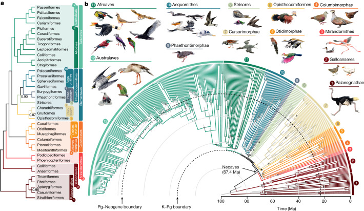
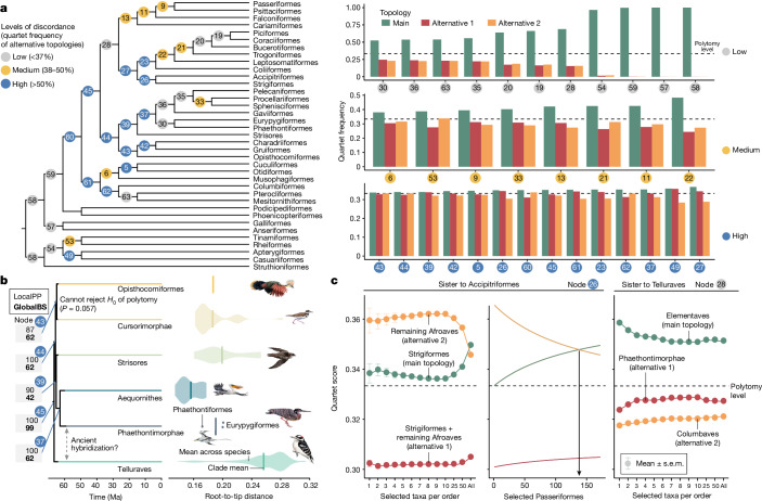
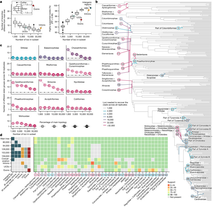
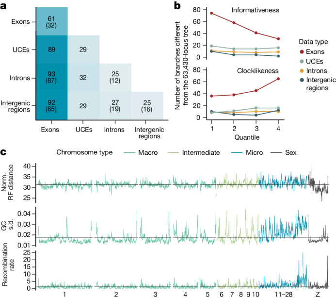
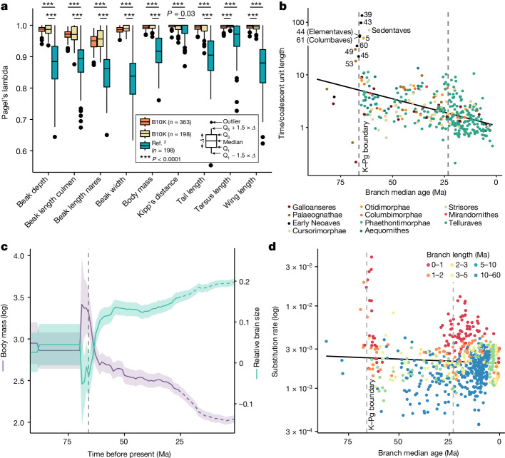
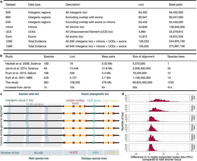
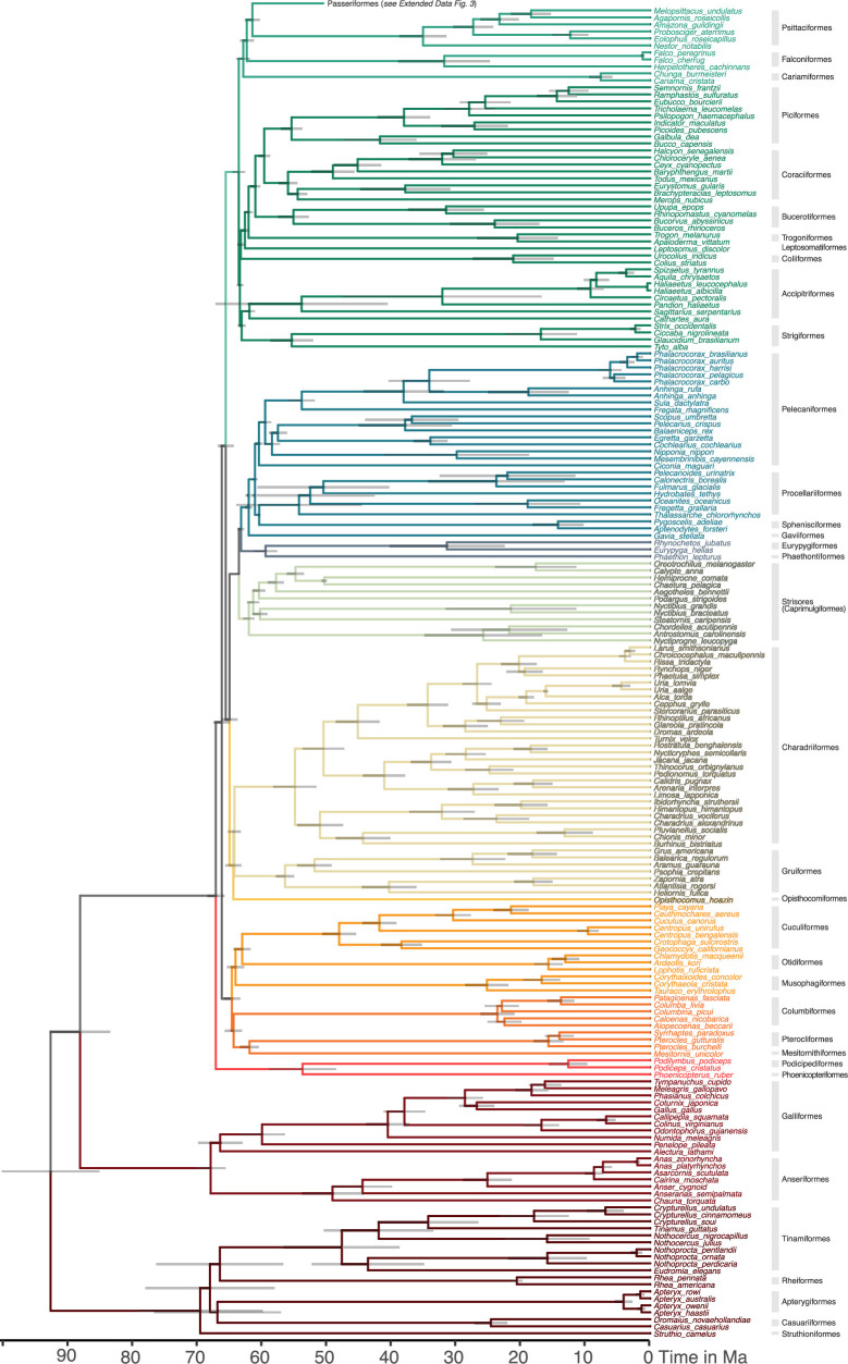
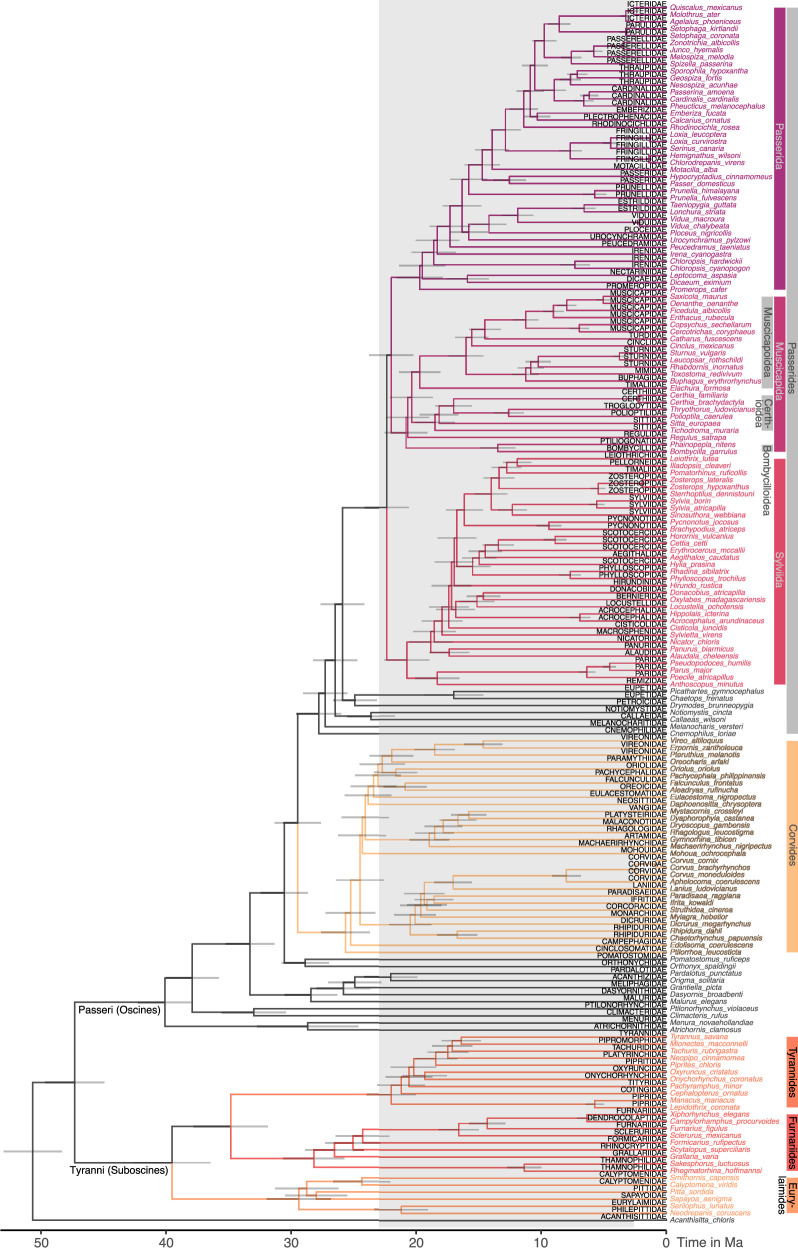
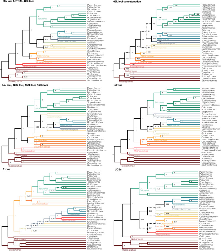
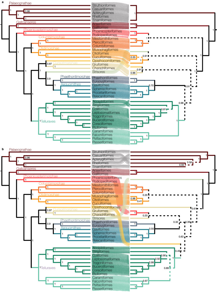
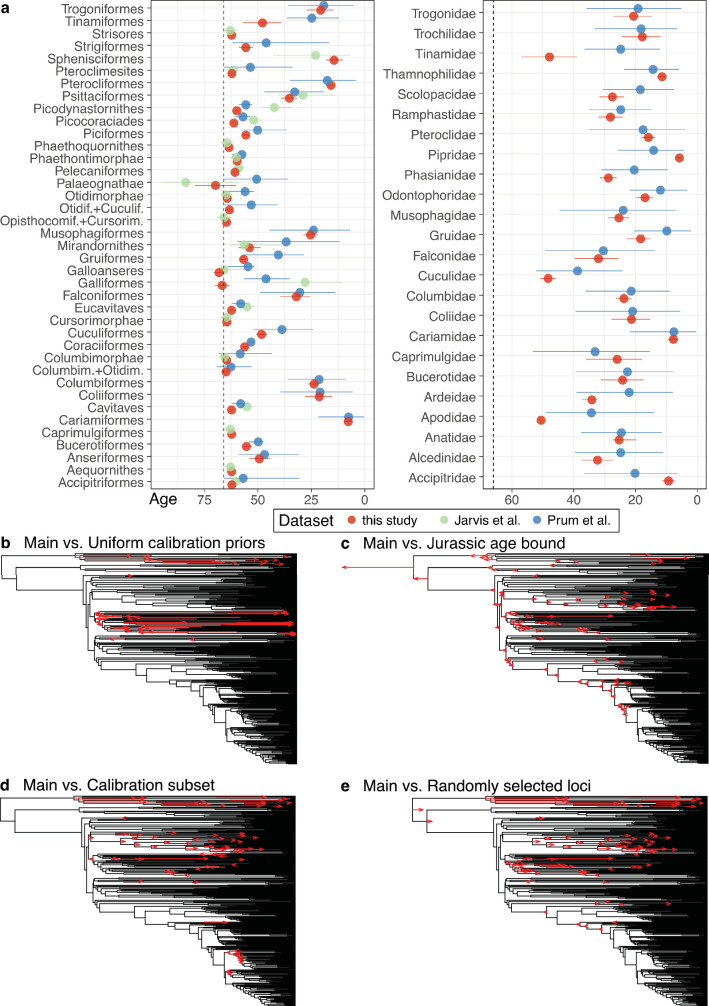
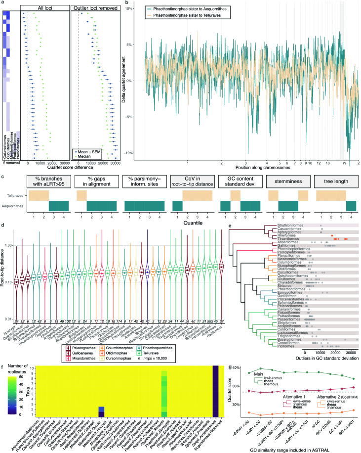
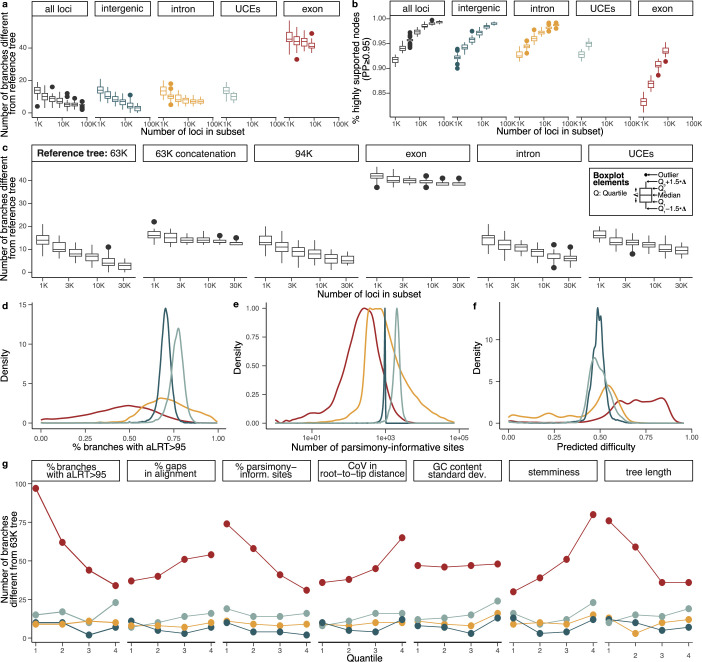
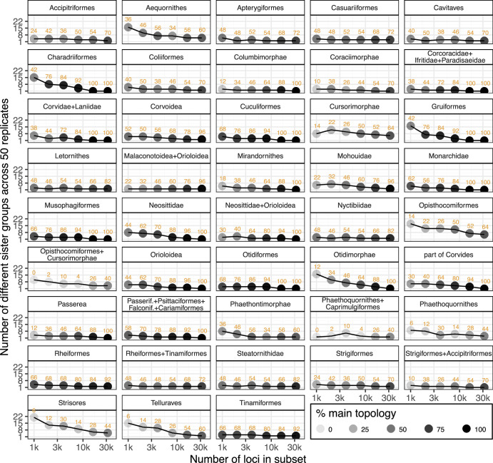
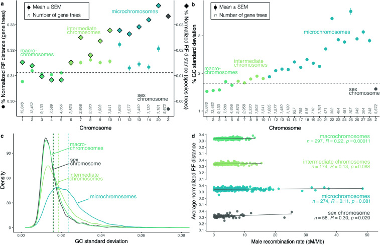
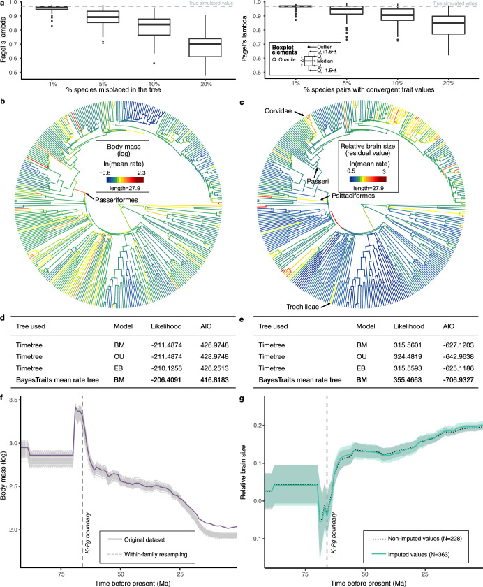
Despite tremendous efforts in the past decades, relationships among main avian lineages remain heavily debated without a clear resolution. Discrepancies have been attributed to diversity of species sampled, phylogenetic method and the choice of genomic regions^1-3. Here we address these issues by analysing the genomes of 363 bird species⁴ (218 taxonomic families, 92% of total). Using intergenic regions and coalescent methods, we present a well-supported tree but also a marked degree of discordance. The tree confirms that Neoaves experienced rapid radiation at or near the Cretaceous-Palaeogene boundary. Sufficient loci rather than extensive taxon sampling were more effective in resolving difficult nodes. Remaining recalcitrant nodes involve species that are a challenge to model due to either extreme DNA composition, variable substitution rates, incomplete lineage sorting or complex evolutionary events such as ancient hybridization. Assessment of the effects of different genomic partitions showed high heterogeneity across the genome. We discovered sharp increases in effective population size, substitution rates and relative brain size following the Cretaceous-Palaeogene extinction event, supporting the hypothesis that emerging ecological opportunities catalysed the diversification of modern birds. The resulting phylogenetic estimate offers fresh insights into the rapid radiation of modern birds and provides a taxon-rich backbone tree for future comparative studies.

Fig. 1. Relationships and divergence times for 363 bird species based on 63,430 intergenic loci.

a, Topology simplified to orders with higher clade names following ref. . Numbers on branches represent local posterior probability if below 1. b, Time tree of all species. Grey bars represent 95% credible intervals for age estimation; dots indicate nodes with fossil calibrations; asterisks mark the three branches lacking full support. A tree with tip labels is shown in Extended Data Figs. 2 and 3.

Fig. 2. Explaining difficult placements.

a, Gene tree discordance across the backbone of the main tree. Node colours and numbers represent the bar plots of quartet frequencies for three possible resolutions around each branch. b, Uncertainty at the base of Elementaves. Phaethontimorphae + Aequornithes had high local posterior probability (LocalPP), but global bootstrap resampling (GlobalBS) showed support for an alternative placement. Violin plots (points for the species-poor Phaethontiformes) show higher root–tip distances of Phaethontiformes, and particularly for Eurypygiformes, than Aequornithes, which may cause attraction to the long-branched Telluraves. Further, the placement of Opisthocomiformes is the only branch where a null hypothesis (H₀) of a polytomy cannot be refuted. c, Addition of taxa occasionally affects topology and support. Across 41,918 GTs with at least one species from each group, the alternative placement of Afroaves + Accipitriformes had higher quartet support when only a few species were sampled but declined with increasing taxon sampling (left), particularly of Passeriformes. The main topology dominated when 138 or more passerines were sampled (middle, arrow). Support for Telluraves + Elementaves decreased with increasing taxon sampling (right). Source Data

Fig. 3. Effect of increasing data quantity.

a–c, Species trees were reconstructed from subsets of GTs (1,000, 2,000, ..., 32,000) of the 63,430 intergenic regions in 50 replicates. a, The addition of loci increases similarity to the main tree (left) and increases the proportion of highly supported nodes (right). b, The main tree, with branches coloured according to the difficulty involved in consistently recovering the clade across subsets. Most branches were consistently obtained with only 1,000 GTs (grey); the remaining 40 branches required more loci. c, Increasing the number of loci decreases the number of possible sister groups. We recorded the number of unique sister groups for each node across subsets. Colours correspond to the difficulty (from b), and shading and number show the frequency, with which the main topology was obtained. The top row illustrates examples of easy nodes. in which the same sister group was consistently recovered with 2,000, 4,000 and 16,000 loci, respectively. The remaining plots show the most difficult nodes, in which multiple sister groups were supported even when 32,000 loci were subsampled. d, Ten selected species trees, data types used in each and the support for all challenging branches (labelled in b). Asterisks indicate relationships in Passeriformes that differ from previous studies. MNO, Malaconotoidea + Neosittidae + Orioloidea; MMNO, Mohouidae + MNO, PP, posterior probability; Q, quartiles. Source Data

Fig. 4. Phylogenetic signal across the genome.

a, Protein-coding regions yield more varied species trees when they are subsampled. Each heatmap cell shows the average Robinson–Foulds distance between 1,250 (diagonal, 1,225) pairs of species trees, each built from 2,000 GTs of different data types. Values in parentheses give the same metrics for 8,000 GTs, omitting UCEs with fewer loci. b, Effect of subsetting loci by data type and different metrics. The y axis represents the number of differences to the main tree; the x axis shows two metrics split into four quartiles, from low to high. Phylogenetic informativeness is the proportion of parsimony-informative sites. Clocklikeness is the coefficient of variation in root–tip distances, a measure of branch length heterogeneity. Extended Data Figure 8g shows other metrics. c, Patterns of phylogenomic incongruence along the genome. Using the 94,402 loci binned approximately every 500 kb, lines show Robinson–Foulds (RF) distances to the main tree (top), variance in GC content (middle) and recombination rate (bottom). Horizontal lines indicate genome-wide averages. Source Data

Fig. 5. Biological implications of the new time tree.

a, The main tree fits morphological traits well. We measured phylogenetic signal (Pagel’s lambda) for nine traits over 100 replicates and compared the fit based on (1) the main tree, (2) the ref. topology and (3) the main tree with random species sampling to match the sample size used in ref. (one-sided t-test with Bonferroni correction). b, The K–Pg and Palaeogene–Neogene transitions were associated with increased effective population sizes of some lineages. Shown are the midpoint ages of each branch compared with the ratio between its length in time units and in coalescent units, which is proportional to the effective population size of that branch and its generation time. Numbers correspond to selected nodes from Fig. 2a. c, Variations in body mass and relative brain size over time changed in different directions following the K–Pg event. Solid lines indicate mean values and ribbons mark 95% confidence intervals. The dashed parts of the reconstruction (from 25 Ma) indicate possible uncertainty due to the lack of within-family sampling (Extended Data Fig. 11g). d, Substitution rates increased around the K–Pg boundary. Estimated molecular rates for the intergenic regions are plotted against the midpoint age of each branch. Source Data

Extended Data Fig. 1. Overview of the phylogenomic dataset.

a, Overview of the datasets by different data types in terms of number of loci and base pairs analyzed. b, Comparison of dataset size to previous studies focused on avian relationships. c, Schematic overview of the extraction of different genomic data types (intergenic regions, exons, UCEs, introns). d, Choice of the length of intergenic loci. To evaluate the impact of locus length of intergenic regions, we used 500 alignments of 10 kb length and extracted subregions of increasing length (0.25 kb to 5 kb) to build gene trees for each. We then calculated the number of well-supported nodes of each locus compared to the next shorter version of the locus. We found that gene tree support increased up to 1 kb length for most loci indicating that phylogenetic signal increased. At lengths greater than 1 kb an increasing number of gene trees had fewer well-supported nodes than at shorter locus lengths (values below 0 in the plot), perhaps due to increasing propensity to include recombinations in a locus. We therefore chose 1 kb as the locus length for our analyses to balance high signal and reduced chance of recombination.

Extended Data Fig. 2. The main dated tree with tip labels for all groups except Passeriformes.

Taxonomic orders are annotated to the right of the tree. Colors of the branches follow those used in Fig. 1. The Passeriformes portion of the tree is shown in Extended Data Fig. 3.

Extended Data Fig. 3. The main dated tree with tip labels for Passeriformes.

Taxonomic family names are given on the branches. Major clades as discussed in the text are annotated to the right following.

Extended Data Fig. 4. Overview of topologies for the species trees obtained for different data types.

Each tree is simplified to taxonomic orders, colors follow those used in Fig. 1. All analyses are coalescent-based species trees obtained from ASTRAL with support being local posterior probabilities, with the exception of the values on the panel showing the topology obtained from concatenated analysis using RAxML-NG with support values resulting from bootstrapping. Poorly supported branches (bootstrap<0.8, local posterior probabilities<0.9) are dashed.

Extended Data Fig. 5. Comparison of the main tree with previous studies simplified to taxonomic orders.

Top, comparison to Jarvis et al. ‘TENT’ on the right. Bottom, comparison with Prum et al. on the right. Bands connect the same tips, dashed branches on the right tree indicate nodes not present in the main tree.

Extended Data Fig. 6. Comparison of inferred ages to previous studies and across alternative analyses.

a, Age estimates in comparison to previous studies for major clades and orders (left) and for families (right). Shown are median age estimates (points) and 95% credible intervals (whiskers) derived from MCMC sampling for clades that were present in at least two studies. The dashed line is the K–Pg boundary. b-e, Comparison of age estimates between the main analysis and alternative analyses. Red arrows indicate the amount of displacement in the date estimates from the main analysis compared with each alternative analysis. For a description of each analysis, refer to the Methods.

Extended Data Fig. 7. Exploration of difficult nodes.

a, Removing species one by one from Columbea and Otidimorphae (rows, heatmap) changed the support for Columbea in the gene trees as measured by the difference between the quartet score of the tree placing Columbea or Mirandornithes at the base. Columbea was not recovered unless all but one Columbiformes or Cuculiformes was removed. Large differences between mean (blue; n = 63,430; shown with s.e.m.) and median (green) show the impact of outlier genes: While the mean score (akin to what is used by ASTRAL) favored Columbea in some cases, the median never favored it. b, Genome-wide scan for the competing topologies for Phaethontimorphae. The main (blue) and the alternative (brown) topology had a normalized quartet score difference of 0.000537%. Chromosomes with <100 windows were excluded. The y axis shows the quartet support for a bipartition in each gene tree minus the mean support for that topology across all gene trees, calculated as a moving average over 100 loci. If a genomic region was strongly in favor of either topology, the two lines would be diverging, but this was not observed. c, The two competing positions (colors as in b) for Phaethontimorphae were responsive to selecting subsets of the intergenic regions that targeted long branches (panels with gray background). Species trees were generated from gene trees split into four quartiles according to their values for seven metrics. For each resulting species tree, the position of Phaethontimorphae is shown (posterior probability=1 throughout). d, Comparison of root-to-tip distances across 21,154,875 gene tree tips as an indicator of susceptibility to long-branch attraction. The violin plots show distributions grouped by orders as well as mean (dots) and three quartiles (horizontal lines). e, Comparison of GC content outliers across birds. For each species grouped by orders, the number of loci that were outliers (defined using the interquartile range) in their GC s.d. from the remaining taxa is shown. The outliers were counted across 159,205 loci from all data types. Rheiformes and Tinamiformes had many loci with a different GC content compared to the remaining birds, which may artificially attract these two taxa. f, Effect of taxon sampling on topology. We sampled 1–10 taxa for each order and investigated the effect on specific nodes, given as the most recent common ancestor (MRCA) of two taxa. Colors indicate the number of replicates that recovered the clade. Most clades were supported irrespective of the number of taxa sampled (yellow), while Columbaves (Mesitornithiformes, Cuculiformes) was only found across all replicates when at least 3 taxa were sampled per order. The MRCA of Phaethontiformes + Strisores was only found when at least 10 taxa were sampled. Strigiformes and Accipitriformes were only recovered as a clade when more than 10 taxa were sampled (discussed in the main text). g, GC-content similarities between Tinamiformes and Rheiformes cause topological changes in gene trees. Positive values of the relative GC similarity indicate that Tinamiformes and Rheiformes are similar to each other but not to Apterygiformes and Casuariiformes, and negative values indicate the opposite. Using this quantity, we divided loci into bins and calculated the quartet score for each bin.

Extended Data Fig. 8. Comparisons between different data types.

Colors are the same for each data type across panels. In panels a–c, 50 subsets were drawn and summarized into species trees for each data type and each subset of n loci. Boxplot components are the same as in c. a, Greater dataset size resulted in increased similarity to the main tree across all data types. b, Greater dataset size resulted in an increased proportion of highly supported nodes of the resulting species tree across all data types. c, Response to increasing dataset size in comparison to different reference species trees. Each panel compares the same subsets of the 63,430 dataset to the reference trees (obtained from summarizing all loci of a data type), showing that increasing gene tree sampling consistently improved similarity. The increase in similarity to the species tree from concatenation and from analyzing exons is less pronounced, indicating more sustained differences despite large numbers of loci. d-f, Density distribution of phylogenetic signal measured as d, the percentage of branches in each gene tree with more than 95% posterior probability support, e, the number of parsimony informative sites (PIS) in a locus, f, the predicted difficulty of each alignment using Pythia. Exons have the lowest signal and are more difficult. UCEs are longer than intergenic regions and thus have more PIS and slightly higher support on average, while the predicted difficulty of estimating trees for both is similar. Introns are heterogenous, ranging from easy to difficult. g, For each data type, loci were sorted according to their magnitude in seven metrics and split into four quantiles. The gene trees of each quantile were summarized into a species tree and compared to the main tree. Exons generally responded the strongest to subsetting, while effects were less pronounced but present in the other data types.

Extended Data Fig. 9. The number of potential sister groups decreases with increasing number of loci.

Only those nodes that still had multiple sister group proposals at 8,000 loci are shown. Points show the number of different sister group proposals obtained across 50 subsets of n loci. Shading of the nodes and orange numbers indicate the proportion with which the main topology was obtained.

Extended Data Fig. 10. Comparison of different chromosomes and chromosomal categories.

a, Discordance across chromosomes. Mean ± s.e.m. of percent normalized Robinson-Foulds (RF) distance for gene trees from the 80,047 locus set derived from individual chromosomes (circles, left y-axis) and absolute RF distance to species trees (diamonds, right y-axis). Dashed line: mean gene tree distance across all chromosomes. Chromosomes with less than 1000 gene trees were not used to construct species trees. b, Mean ± s.e.m. of the GC s.d. of gene trees from the 80,047 locus set for each chromosome, showing a general increase in GC s.d. in shorter chromosomes. Dashed line: mean across all chromosomes. c, Density plot for distribution of GC s.d. for alignments, showing higher deviation for microchromosomes. d, Pearson correlation of mean normalized RF distance and recombination rate for loci of different chromosome types binned over 500 kb. No adjustments for multiple comparisons were made.

Extended Data Fig. 11. Trait evolution.

a, Simulations on inferred Pagel’s lambda (λ) values. To simulate topological error (left), continuous traits were simulated and an increasing proportion of species were randomly misplaced in the phylogeny (n = 100). To simulate the effect of convergence in trait values (right), continuous traits were simulated on a phylogeny and an increasing proportion of species pairs were randomly given the same trait value to simulate the action of convergence (n = 100). Compared to the effects of topological inaccuracies, the influence of convergently similar trait values on λ estimates was weaker. b, Reconstruction of rate changes in body mass evolution (log-transformed). Branches are colored by estimates of the mean rate (log-transformed); rate changes can occur in both directions, either an increase or a decrease. c, Reconstruction of rate changes in relative brain size evolution (residual). Branch colors as in b. Taxa with pronounced rate changes as mentioned in the main text are annotated. d, Model comparisons between variable-rate and single-process models (BM: Brownian motion, EB: early burst, OU: Ornstein–Uhlenbeck) for body size. e, Model comparisons as in d for relative brain size. f, Impact of taxon sampling on ancestral reconstruction of body size. The solid purple line is the result of the ancestral reconstruction of the full dataset. The gray lines are ancestral reconstructions from analyses in which each species’ trait values were randomly drawn from the range of values across their family (n = 100). The chosen values did not impact the reconstructions at deep timescales but estimates diverged more from 25 million years ago to the present, indicating that increased taxon sampling within families may lead to a different trajectory in more recent times. g, Impact of imputation on ancestral reconstructions of relative brain size. The non-imputed dataset contained only values based on the literature, while the imputed dataset included some values inferred using phylogenetic information. Solid lines indicate mean values and ribbons mark 95% confidence intervals. The two ancestral reconstructions are almost indistinguishable.

References

1. Jarvis ED, et al. Whole-genome analyses resolve early branches in the tree of life of modern birds. Science. 2014;346:1320–1331. doi: 10.1126/science.1253451. - DOI - PMC - PubMed
1. Prum RO, et al. A comprehensive phylogeny of birds (Aves) using targeted next-generation DNA sequencing. Nature. 2015;526:569–573. doi: 10.1038/nature15697. - DOI - PubMed
1. Kuhl H, et al. An unbiased molecular approach using 3’-UTRs resolves the avian family-level Tree of Life. Mol. Biol. Evol. 2021;38:108–127. doi: 10.1093/molbev/msaa191. - DOI - PMC - PubMed
1. Feng S, et al. Dense sampling of bird diversity increases power of comparative genomics. Nature. 2020;587:252–257. doi: 10.1038/s41586-020-2873-9. - DOI - PMC - PubMed
1. Hinchliff CE, et al. Synthesis of phylogeny and taxonomy into a comprehensive tree of life. Proc. Natl Acad. Sci. USA. 2015;112:12764–12769. doi: 10.1073/pnas.1423041112. - DOI - PMC - PubMed