Time-series reconstruction of the molecular architecture of human centriole assembly

Abstract

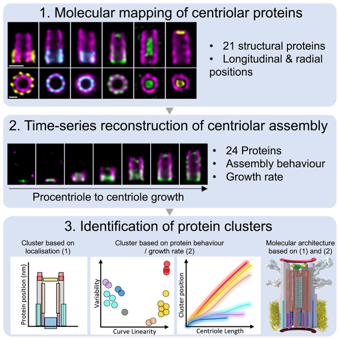
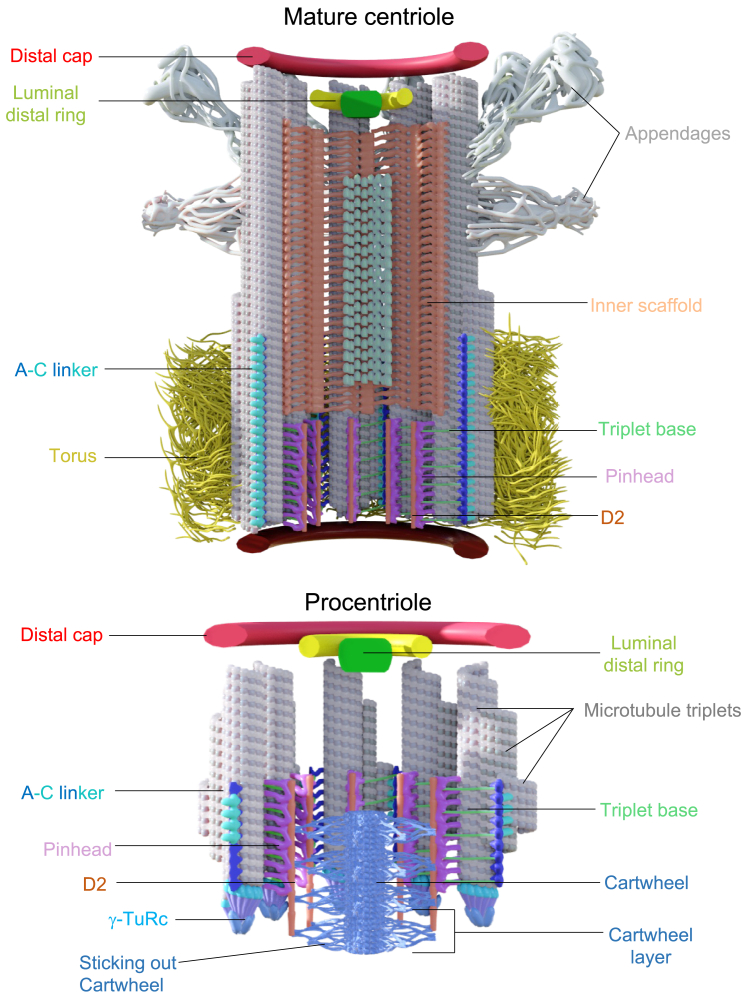
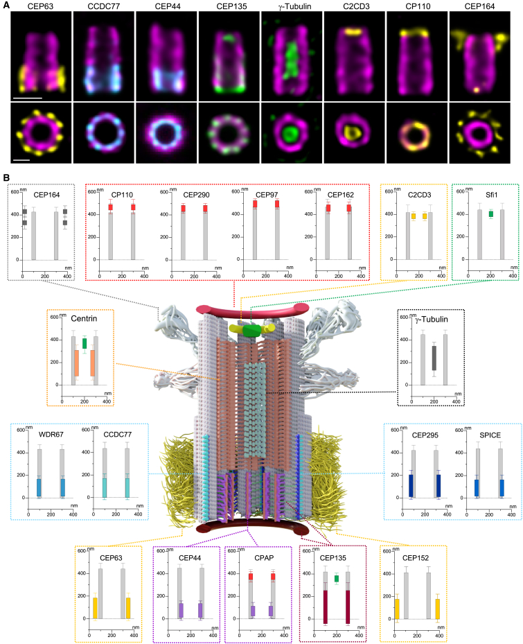
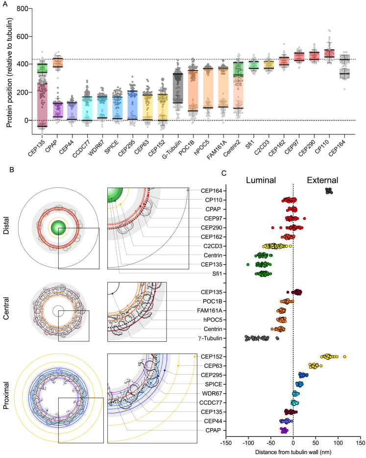
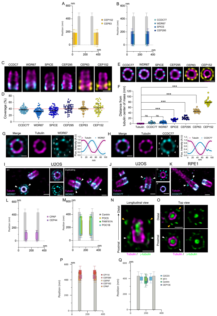
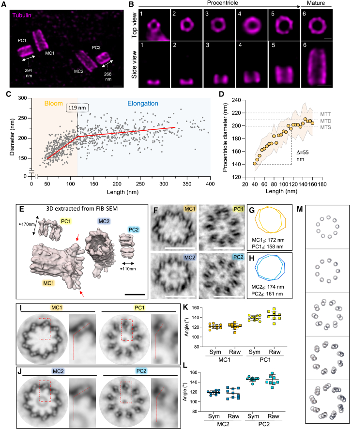
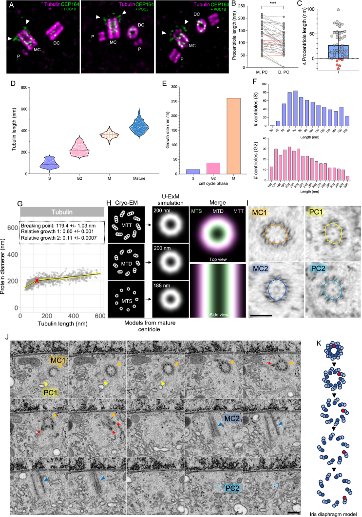
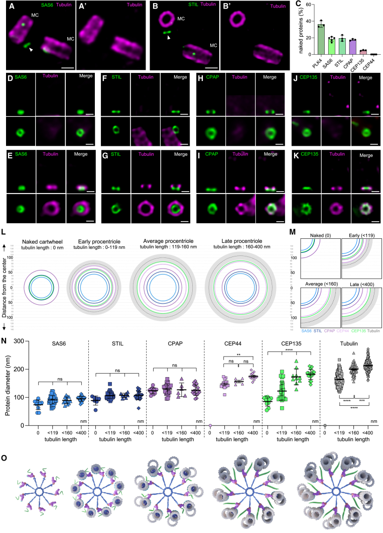
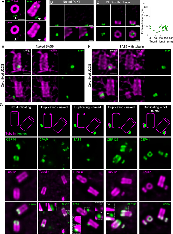
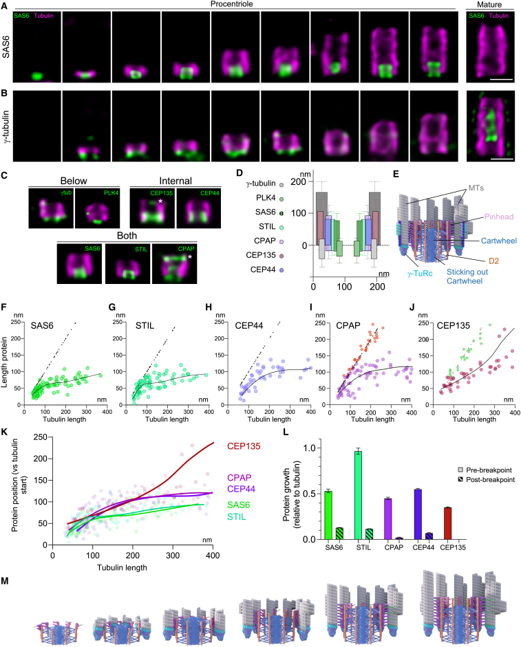
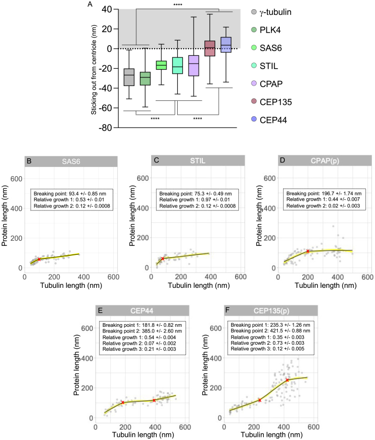
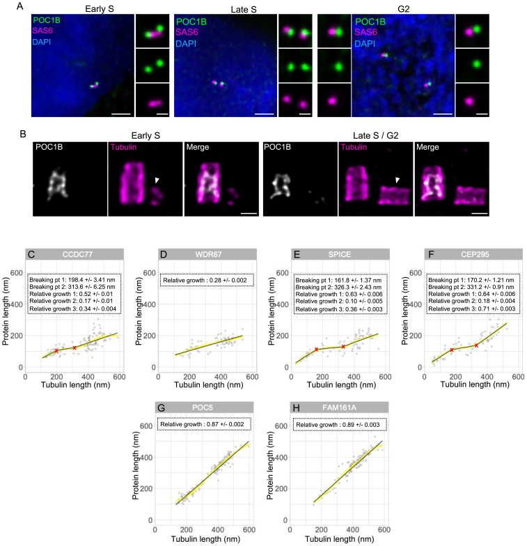
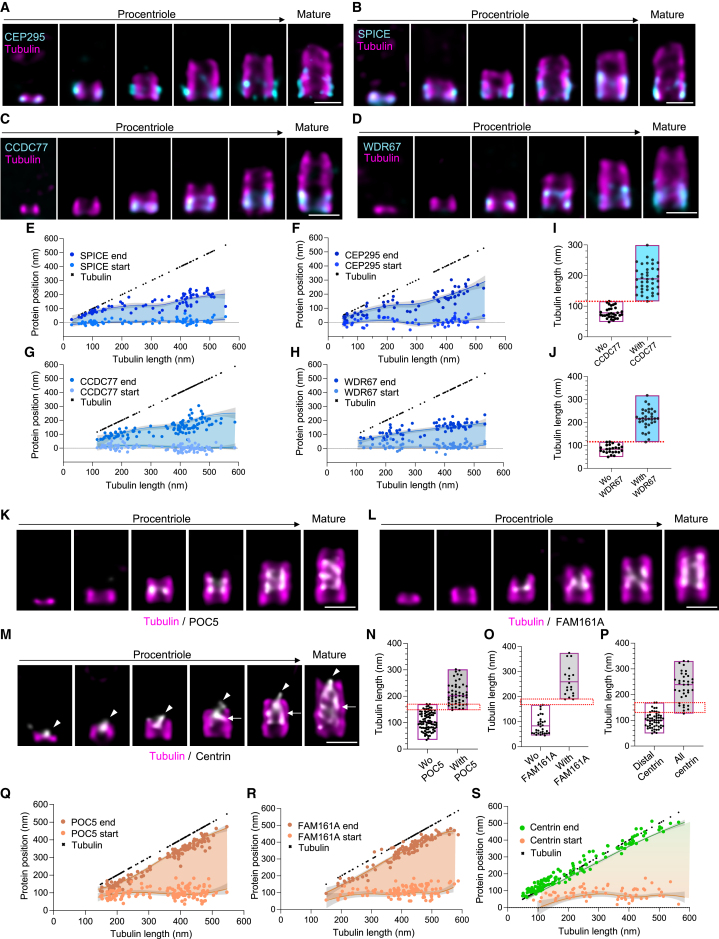
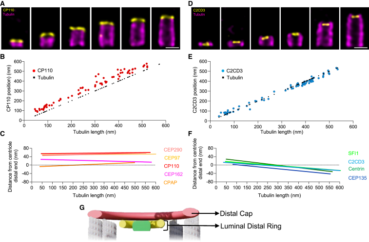
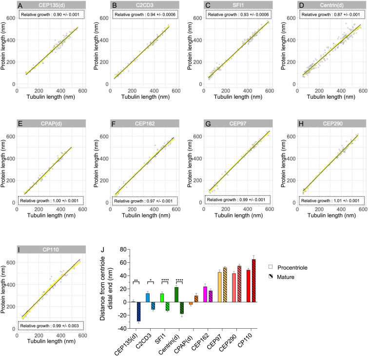
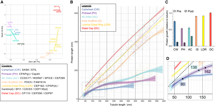
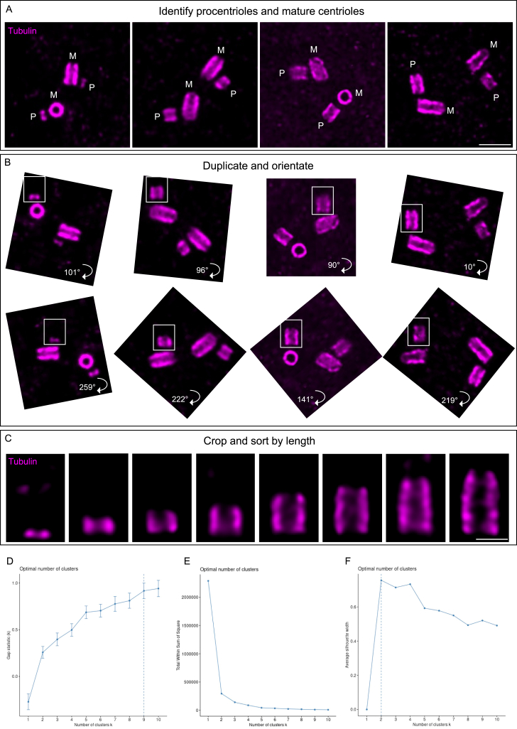
Centriole biogenesis, as in most organelle assemblies, involves the sequential recruitment of sub-structural elements that will support its function. To uncover this process, we correlated the spatial location of 24 centriolar proteins with structural features using expansion microscopy. A time-series reconstruction of protein distributions throughout human procentriole assembly unveiled the molecular architecture of the centriole biogenesis steps. We found that the process initiates with the formation of a naked cartwheel devoid of microtubules. Next, the bloom phase progresses with microtubule blade assembly, concomitantly with radial separation and rapid cartwheel growth. In the subsequent elongation phase, the tubulin backbone grows linearly with the recruitment of the A-C linker, followed by proteins of the inner scaffold (IS). By following six structural modules, we modeled 4D assembly of the human centriole. Collectively, this work provides a framework to investigate the spatial and temporal assembly of large macromolecules.

Keywords: centriole assembly; centriole duplication; centrioles; expansion microscopy; molecular mapping; super-resolution microscopy; time-series reconstruction.

Graphical abstract

Figure S1

Index of centriole structures, related to Figure 1 Scheme of the procentriole and mature centriole structural elements and their corresponding legends.

Figure 1

Nanoscale mapping of 21 proteins in human mature centrioles (A) Centrioles observed in side view (top) or top view (bottom). Cells were stained for tubulin (magenta) and CEP63, CCDC77, CEP44, CEP135, γ-tubulin, C2CD3, CP110, and CEP164. Scale bars: 200 (top) and 100 (bottom) nm. (B) Model of a human mature centriole displaying the structural elements of the centriole along its proximal to distal axis. MTT, gray; pinhead, magenta; triplet base, green chartreuse; A-C linker, cyan; torus, dark yellow; inner scaffold, orange peach; luminal tube, light green; luminal distal ring, green/yellow; distal cap, red; appendages, white. The radial and longitudinal positions of each protein along the centriole are depicted next to the model. Error bars denote SD. See Table S2 for statistics. See also Figures S1, S2, and S3.

Figure S2

Mapping the human mature centrioles by U-ExM, related to Figure 1 (A) Longitudinal positions of the 21 mapped proteins relative to the normalized tubulin signal. Black dotted lines indicate the start and the end of the tubulin signal, depicting the centriole length. For each protein, the start (light gray dots) and end (dark gray dots) position of the fluorescent signal is presented. Note that for the distal proteins only present as a thin layer, one unique peak of fluorescence could be detected, and, therefore, the measurement reflects the thickness of the fluorescence signal around the peak. Each filled color bar represents the coverage of the indicated protein inside the centriole. See Table S2 for statistics. (B) Graphical representation of the radial positions of the 21 mapped proteins relative to the tubulin signal, juxtaposed to a cryo-EM map of a Chlamydomonas centriole. Black dotted circles indicate the tubulin signal, depicting the MTT wall diameter in the proximal, central, and distal regions. Each color circle corresponds to the diameter of the indicated protein based on measurements presented in (C) and normalized on the average tubulin diameter at each specific region (see STAR Methods). Tubulin diameter (average ± SD): proximal = 197 ± 15 nm; central = 181 ± 13 nm; distal = 167 ± 22 nm. n = 26, 20, and 24 centrioles from three independent experiments for proximal, central, and distal, respectively. See Table S2 for statistics. (C) Distance between the MTT wall (tubulin signal) and the indicated proteins (in nm). A distance below 0 indicates that the protein is localized inside the centriole, while a distance above 0 indicates a protein that is localized outside the centriole. See Table S2 for statistics.

Figure S3

Detailed features of protein clusters in human mature centrioles, related to Figure 1 (A) Overlapping radial and longitudinal positions of the torus components, CEP63 (yellow) and CEP152 (mustard), relative to tubulin signal (gray). See Table S2 for statistics. (B) Overlapping radial and longitudinal positions of the A-C linker candidates CCDC77, WDR67, SPICE, and CEP295 (light blue to dark blue) relative to tubulin signal (gray). See Table S2 for statistics. (C) Side views of centrioles from U2OS cells stained for tubulin (magenta) and, from left to right, CCDC77, WDR67, SPICE, CEP295, CEP6, and CEP152. Scale bars: 200 nm. (D) Coverage of indicated protein, expressed as a percentage of the tubulin length. Average ± SD are as follows: CCDC77 = 37.2% ± 7.4%, WDR67 = 32.1% ± 9.0%, SPICE = 34.3% ± 9.7%, CEP295 = 41.8% ± 12.6%, CEP63 = 41.5% ± 10.2%, and CEP152 = 43.3% ± 14.0%. n = 70, 81, 76, 48, 70, and 57 centrioles for CCDC77, WDR67, SPICE, CEP295, CEP63, and CEP152, respectively. (E) Top views of centrioles stained for tubulin (magenta) and, from left to right, CCDC77, WDR67, SPICE, CEP295, CEP63, and CEP152. Scale bars, 100 nm. (F) Distance between the tubulin signal and the indicated protein signal. Average ± SD are as follows: tubulin = 0 ± 0 nm, CCDC77 = 2.6 ± 3.1 nm, WDR67 = 5.2 ± 3.0 nm, SPICE = 14.5 ± 3.5 nm, CEP295 = 21.7 ± 5.8 nm, CEP63 = 46.7 ± 6.3 nm, and CEP152 = 79.6 ± 10.3 nm. n = 28, 18, 19, 14, 18, 19, and 25 centrioles for tubulin, CCDC77, WDR67, SPICE, CEP295, CEP63, and CEP152, respectively. (G and H) Centrioles from top view stained for tubulin (G and H) and WDR67 (G) or CCDC77 (H). Note that both WDR67 and CCDC77 are located in between each microtubule triplet visualized thanks to tubulin staining. Fluorescence intensity profile along two successive MTTs demonstrating the precise position of WDR67 (G) and CCDC77 (H) are shown on the right of the figures. (I) Centrosomes stained for tubulin and WDR67 showing a torus-like localization of the protein (white arrowheads), on top of its A-C linker localization. Note that this torus-like pattern is present at only one centriole in G1 and at both once centrioles start to duplicate, reminiscent of the behavior of the torus proteins CEP63 and CEP152. Scale bars: 200 nm. (J) Centrosomes stained for tubulin and CCDC77 showing an additional localization toward the distal end of the centriole, organized in a 9-fold symmetry outside the tubulin wall (white arrowheads). Note that this additional localization is only present at one of the two mature centrioles. Scale bars: 200 nm. (K) Centrioles from ciliated RPE1, stained for tubulin and CCDC77, showing the additional localization of CCDC77 at the distal end of the basal body undergoing ciliogenesis (white arrowheads). Scale bars: 200 nm. (L) Overlapping radial and longitudinal positions of the pinhead components, CPAP (mauve) and CEP44 (purple), relative to tubulin signal (gray). See Table S2 for statistics. (M) Overlapping radial and longitudinal positions of the inner scaffold components centrin (dark gray), POC5 (yellow), FAM161A (green), and POC1B (blue) relative to tubulin signal (gray). See Table S2 for statistics. (N and O) Centrioles from U2OS cells stained for tubulin and γ-tubulin, observed from side view (N) and from top view (O). γ-tubulin is located both in the lumen of the centriole and around the centriole, with two distinct localizations in the proximal (white arrowheads) and distal (yellow arrowheads) regions. Scale bars: 200 nm (N) and 100 nm (O). (P) Overlapping radial and longitudinal positions of the distal cap components CP110 (red), CEP290 (light red), CEP97 (yellow), CEP162 (pink), and CPAP (orange) relative to tubulin signal (gray). See Table S2 for detailed statistics. (Q) Overlapping radial and longitudinal positions of the luminal distal ring components C2CD3 (light blue), SFI1 (light green), centrin (dark green), and CEP135 (dark blue) relative to tubulin signal (gray). See Table S2 for statistics.

Figure 2

Monitoring the growth of the centriolar microtubule wall (A) Centrosomes from duplicating cell stained for tubulin. Note the asymmetry of procentriole length (PC1 > PC2 of 26 nm). MC, mature centriole; PC, procentriole. Scale bars: 200 nm. (B) Centrioles stained for tubulin observed in top view (top) and in side view (bottom). Scale bars: 100 (top) and 200 (bottom) nm. (C) Evolution of the tubulin diameter over length during procentriole to mature centriole assembly. Measurements of 829 centrioles from >10 independent experiments were fitted with a segmented linear regression (see Figure S4G). (D) Evolution of the tubulin diameter over length during the early stages of procentriole assembly. Gray dashed lines indicate the simulated diameters of mature centrioles with microtubule singlets (MTSs), microtubule doublets (MTDs), and microtubule triplets (MTTs) based on cryoelectron microscopy (cryo-EM) image (see Figure S4H). (E) 3D representation of a HeLa centrosome focus ion beam - scanning electron microscopy (FIB-SEM) image (from https://openorganelle.janelia.org/datasets/jrc_hela-2). Note the asymmetry of procentriole length (PC1 > PC2 of 60 nm). Red arrows indicate distal appendages of the mature centriole (MC1). Scale bars: 200 nm. (F) Top views of the mature centrioles and procentrioles. Scale bars: 200 nm. (G and H) Diameter representation from MC1/PC1 (G, orange/yellow) and MC2/PC2 (H, dark blue/light blue) measured from images in (F). (I and J) Circularized and symmetrized images from (F). (K and L) MTT/MTD angles measured from raw (F) and symmetrized (I and J) images from MC1/PC1 (K) and MC2/PC2 (L). See Table S2 for statistics. (M) Model of the procentriole bloom with the sequential appearance of the A-, B-, and C-microtubules. See also Figure S4.

Figure S4

Monitoring the growth of the centriolar microtubule wall, related to Figure 2 (A) Centrosomes from duplicating U2OS stained for tubulin and the distal appendages marker CEP164 (white arrowheads) and either POC1B or POC5 (inside the centrioles). As CEP164 is only present when the centriole reaches its final mature stage, it allows us to distinguish mother and daughter centrioles. Images show a systematic asymmetry of the procentriole length toward the mother centriole. Scale bars: 200 nm. (B) Procentriole length growing from the mother (M. PC) or the daughter (D. PC) centriole showing a significant length asymmetry between the two procentrioles. ^∗∗∗p < 0001, paired Student’s t test. n = 50 centrioles from >3 independent experiments. (C) Procentriole length difference (delta) from each pair of centrosomes measured. Average ± SD: 27.2 ± 27.4 nm. n = 50 centrioles from >3 independent experiments. (D–F) Procentriole growth estimation through cell-cycle phases. (D) Centriole length distribution through the different stages of the cell cycle (procentrioles during S phase, G2, mitosis, and mature centrioles), showing the constant increase in length. Given that POC5-positive procentrioles are typically found in the G2 phase, procentrioles smaller than 160 nm, devoid of POC5 staining (Figure 5N), are thus presumed to be in the S phase. Average ± SD are as follow: S = 94.66 ± 32.73 nm, G2 = 228.4 ± 44.7 nm, M = 359.3 ± 25.64 nm, mature = 438.9 ± 47.42 nm. n = 656, 352, 62, and 798 centrioles for S, G2, M, and mature, respectively, from >5 independent experiments. (E) Growth rate of procentrioles during S phase, G2, and mitosis, based on data from (A). Growth rate in nm/h: S = 15.81 nm/h, G2 = 38.61 nm/h, and M = 261.4 nm/h. The difference between the maximum and minimum centriole length in each cell-cycle phase divided by the phase duration, allows us to calculate the growth rate (nm/h), demonstrating a difference of growth rate between S, G2, and mitosis. (F) Histogram distribution of procentriole according to their length during S phase (purple) and G2 phase (pink). n = 656 (S) and 352 (G2) centrioles per condition. (G) Plot of loess fit (yellow) compared with a segmented linear regression (black line), with one breakpoint showing a phase of diameter and length growth at a near-linear rate (slope of 0.60 ± 2 × 0.0005). This phase, called bloom phase, stops when tubulin length reaches 119 nm and a second phase of elongation starts at a lower rate (slope of 0.11 ± 2 × 0.0003). In the box are the breakpoint location (red cross) and the slopes (relative growth) of the two segments, along with their respective standard errors. The superposition shows that the segmented regression is a good representation of the overall growth. (H) Model of a Chlamydomonas mature centriole extracted from a cryo-EM image, represented with triplet (top), doublet (middle), or singlet (bottom) microtubules. Images were scaled down to mimic a fluorescent signal of expanded centrioles, and the diameters of each representation were measured. Right panel shows the merge of the three representations in top view and side view (MTT, microtubule triplet, pink; MTD, microtubules doublet, white; MTS, microtubule singlet, green). (I) Extracted images from the raw image (see D) of mature centrioles (MC1 and MC2) and procentrioles (PC1 and PC2) in top views. Each image is superimposed with the nine-sided polygon used to calculate the mean diameter of the ellipse passing through each A-microtubule (see Figure 2G). Scale bars: 200 nm. (J) Image montage of the raw FIB-SEM (from https://openorganelle.janelia.org/datasets/jrc_hela-2) in the centrosome region, allowing us to visualize the two mature centrioles (MC1, orange; MC2, blue) with their respective procentrioles (PC1, yellow; PC2, blue). Note the presence of distal appendages (red arrows) on the mature centriole 1, indicating that it is the mother. Scale bar: 200 nm. (K) Scheme of the iris diaphragm model from Albrecht-Buehler.

Figure 3

Steps of procentriole initiation (A–B′) Centrosomes stained for tubulin and SAS-6 (A and A′) or STIL (B and B′). Arrowheads indicate the presence of SAS-6 (A) and STIL (B) in absence of tubulin signal (A′ and B′), thereafter called “naked.” MC, mature centriole. Scale bars: 200 nm. (C) Percentage of cells presenting a signal for PLK4, SAS-6, STIL, CPAP, CEP135, and CEP44 at the level of the future procentriole in the absence of a tubulin signal. See Table S2 for statistics. (D–K) Procentrioles stained for tubulin and SAS-6 (D and E), STIL (F and G), CPAP (H and I), and CEP135 (J and K). (D), (F), (H), and (J) show naked SAS-6, STIL, CPAP, and CEP135, and (E), (G), (I), and (K) show the protein in early procentrioles. Scale bars: 100 nm. (L and M) Normalized diameter representation of SAS-6 (light blue), STIL (dark blue), CPAP (purple), CEP44 (mauve), and CEP135 (green) at different stages of procentriole assembly according to the tubulin (gray) length (0, <119, <160, and <400 nm). All diameters were normalized on the average tubulin diameter. See Table S2 for detailed statistics. (N) Raw diameters of SAS-6, STIL, CPAP, CEP44, and CEP135 at the same stages of procentriole assembly as in (M). See Table S2 for statistics. (O) Model of the structural reorganization of the cartwheel during the bloom phase. Initially, the cartwheel is formed with SAS-6 and STIL, and part of the pinhead and D2 density (CPAP). A-microtubules appear with the triplet base (CEP135). The microtubule blades separate from each other, reorganizing the pinhead and triplet base until the procentriole is completely formed before the end of the bloom phase. See also Figure S5.

Figure S5

Methodology of the naked cartwheel observation, related to Figure 3 (A) Overexposed image presented in Figures 3A and 3B showing the presence of STIL (left, white arrowhead) and SAS-6 (right, white arrowhead) in absence of tubulin signal. Scale bars: 200 nm. (B and C) Procentrioles stained for tubulin (magenta) and PLK4 (green). Note that (B) shows the presence of PLK4 at the level of the future centriole without the tubulin signal (naked), and (C) shows the early procentriole where the PLK4 signal can be found at the level of a tubulin-positive procentriole. Scale bars: 100 nm. (D) PLK4 diameter evolution during centriole assembly (relative to tubulin length), showing no increase in PLK4 diameter. (E and F) Centrioles from cryo-fixed U2OS cells stained for tubulin and SAS-6. (E) shows the presence of SAS-6 at the level of the future centriole without the tubulin signal, and (C) shows the early procentriole where SAS-6 signal is found at the level of a tubulin-positive procentriole. Scale bars: 200 nm. (G) Examples of widefield images used for the quantification of the percentage of cell with naked proteins (Figure 3C). Top panel shows a graphical representation of each situation (“not duplicating,” “duplicating—naked,” and “duplicating not naked”). Middle and bottom panels show representative images of each situation. Dashed squares indicate overexposed zoom in, showing the absence of tubulin in the naked situation. Scale bars: 250 nm.

Figure 4

Procentriole elongation (A and B) Centrioles during assembly and at mature stage stained for tubulin (A) and (B) and SAS-6 (A) or γ-tubulin (B). Scale bars: 200 nm. (C) “Average” procentrioles (180–200 nm in length) stained for tubulin and γ-tubulin, PLK4, CEP135, CEP44, SAS-6, STIL, and CPAP. Asterisks indicate additional distal localization of CPAP and CEP135. (D) Relative protein longitudinal and radial positions compared with tubulin. See Table S2 for statistics. (E) Structural model of the procentriole, lateral view. (F–J) Evolution of SAS-6 (F), STIL (G), CEP44 (H), CPAP (I), and CEP135 (J) length over tubulin growth during procentriole assembly. CPAP and CEP135 present a dual localization in the proximal (CPAP purple and CEP135 dark red) and distal (CPAP red and CEP135 green) regions. This figure focuses on the proximal localization (see Figure 6 for distal analysis). The evolution of each set of data was represented as loess curves (black line) to estimate the behavior of each protein during their growth (relative to tubulin). (K) Merged data from graphs (F) to (J) with the dot plots and the loess curves for each protein, showing three main clusters based on their similar behaviors (SAS-6/STIL, CPAP/CEP44, and CEP135). The breakpoints, when the growth rates change significantly, are indicated in Figure S6. (L) Protein growth rate relative to tubulin growth before (plain bars) and after (striped bars) breakpoint. See Table S2 for statistics. (M) Model of the formation and elongation of the cartwheel and procentriole during the bloom phase. A cartwheel layer assembles before γ-TuRC recruitment and microtubule blade assembly. The microtubules elongate approximately two times faster than the cartwheel structures, the pinhead, the D2 density, and the triplet base. During assembly, a cartwheel layer is always lower than the microtubules. After about 100 nm of cartwheel elongation, it stops growing, in contrast to the pinhead and D2 density, which grows to about 190 nm. See also Figure S6.

Figure S6

Growth rate of the cartwheel and pinhead components, related to Figure 4 (A) Distance between protein signal and tubulin signal start (sticking out). Average ± SD are as follows: PLK4 = −30.59 ± 12.5 nm, γ-tub = −28.25 ± 11.2 nm, SAS-6 = −16.72 ± 8.2 nm, STIL = −17.72 ± 11.3 nm, CPAP = −13.93 ± 16.6, CEP135 = −0.37 ± 13.7 nm, and CEP44 = 2.36 ± 11.6 nm. n = 38, 28, 79, 81, 58, 57, and 41 centrioles for γ-tub, PLK4, SAS-6, STIL, CPAP, CEP135, and CEP44, respectively, from three independent experiments. Statistical differences were assessed using a one-way ANOVA followed by Tukey’s post hoc test. ^∗∗∗∗p < 0.0001 in all conditions tested. (B–F) Plots of loess fits and superimposed segmented regressions per protein showing that the segmented regressions are a good representation of the overall data (as in Figure S4D).

Figure S7

Characteristics of the MTT connectors, related to Figure 5 (A) Non-expanded U2OS stained for POC1B (green; dilution 1:500), SAS-6 (magenta; dilution 1:100), and DAPI (blue) during cell-cycle progression. Images show no colocalization between SAS-6 (procentriole marker) and POC1B, indicating that POC1B is only present at mature centrioles. Scale bars: 2 μm and 500 nm (inset). (B) Centrioles from expanded U2OS stained for tubulin and POC1B during cell-cycle progression. Note that expansion confirmed that POC1B is only present at the level of mature centrioles and not at procentrioles. Scale bars: 200 nm. (C–F) Plots of loess fits and superimposed segmented regressions per protein showing that the segmented regressions are a good representation of the overall data (as in Figure S4D). (G and H) Plots of loess fits and superimposed segmented regressions per protein, showing that the segmented regressions are a good representation of the overall data (as in Figure S4D).

Figure 5

The MTT connectors assembly (A–D) Procentrioles during assembly and mature centriole stained for tubulin and CEP295 (A), SPICE (B), CCDC77 (C), and WDR67 (D). Scale bars: 200 nm. (E–H) Evolution of the start and end position of SPICE (E), CEP295 (F), CCDC77 (G), and WDR67 (H) signals relative to tubulin growth during procentriole assembly. The growth of each protein was represented as loess curves (blue lines). The light blue region depicts the region of the centriole that is covered by the protein signal. (I and J) Centriole length, based on the tubulin signal, with and without (Wo) CCDC77 (I) or WDR67 (J). The dotted red line represents the average tubulin length when the CCDC77 and WDR67 signal appears (≈115 nm). See Table S2 for statistics. (K–M) Procentrioles during assembly and mature centriole stained for tubulin and POC5 (K), FAM161A (L), and centrin (M). Arrowheads and arrows indicate the luminal distal localization and the microtubule-associated central localization of centrin, respectively (M). Scale bars: 200 nm. (N–P) Centriole length with and without (Wo) POC5 (N), FAM161A (O), and central centrin (P). The dotted red square represents the average tubulin length when POC5, FAM161A, and central centrin signals appear (≈160, 170, and 150 nm, respectively). See Table S2 for statistics. (Q–S) Evolution of the start and end position of POC5 (Q), FAM161A (R), and centrin (S) signals relative to tubulin growth during procentriole assembly. The growth of each protein was represented as loess curves (green/orange lines). The peach/peach-to-green regions depict the region of the centriole that is covered by POC5, FAM161A, or centrin signals. See also Figure S7.

Figure 6

Two distal complex rings (A) Procentrioles during assembly and mature centriole stained for tubulin and CP110. Scale bars: 200 nm. (B) Evolution of CP110 position signal relative to tubulin growth during procentriole assembly. (C) Linear regression curves showing the position of the distal proteins CEP290, CEP97, CP110, CEP162, and CPAP-distal, relative to the end of the tubulin signal during centriole assembly. (D) Procentrioles during assembly and mature centriole stained for tubulin and C2CD3. Scale bars: 200 nm. (E) Evolution of position of C2CD3 signal relative to tubulin growth during procentriole assembly. (F) Linear regression curves showing the position of the distal proteins SFI1, C2CD3, centrin-distal, and CEP135-distal relative to the end of the tubulin signal during centriole assembly. (G) Model of the structures present at the distal level of the centriole, the distal cap (red) that comprises proteins that localize on the plus end of microtubule triplets, and the luminal distal ring (green and yellow). See also Figure S8.

Figure S8

Characteristics of the distal proteins, related to Figure 6 (A–I) Plots of loess fits and superimposed segmented regressions per protein, showing that the segmented regressions are a good representation of the overall data (as in Figure S4D). (J) Distance between the indicated proteins and the end of the centriole, assessed by the tubulin signal. Negative values indicate that the protein ends before the end of the centriole, while positive values indicate that the protein sticks out from the centriole. Plain bars depict the measurements done on procentrioles, striped bars depict measurements on mature centrioles. CEP135(d) procentriole vs. mature centriole: ^∗∗p = 0.002; C2CD3 procentriole vs. mature centriole: ^∗p = 0.012; SFI1 procentriole vs. mature centriole: ^∗∗∗p < 0.0001; centrin(d) procentriole vs. mature centriole: ^∗∗∗p < 0.0001, Kruskal-Wallis followed by Dunn’s post hoc test. See Table S2 for statistics.

Figure 7

Choreography of the molecular architecture of centriole biogenesis (A) Clustering of the 20 proteins exhibiting a quantifiable growth during centriole assembly based on their average growth curves’ distance. The x axis separates growth based on their linearity from nonlinear (left) to near-linear growth (right), while the y axis describes the amount of deviation. The clusters formed by statistical analyses matched with centriolar structural elements, named as follows: cartwheel (SAS-6 and STIL), pinhead (CPAPp and CEP44), A-C linker (CCDC77, WDR67, SPICE, and CEP295), inner scaffold (POC5 and FAM161A), luminal distal ring (CEP135p, SFI1, centrin, C2CD3, CPAPd, and CEP162), and distal cap (CEP97, CEP290, and CP110). Note the individual behavior of CEP135p, which could not be associated with any clusters. (B) Fits of loess regressions with confidence bands for the clusters in (A). The dotted black line corresponds to the tubulin, exhibiting an exact linear growth (slope = 1). The graph highlights the clear separation between the nonlinear growth clusters (cartwheel, pinhead, and A-C linker) and near-linear growth clusters (inner scaffold, luminal distal ring, and distal cap). (C) Chart graph showing the average growth rate for each cluster prior to and after the breakpoints calculated from loess curves (B). (D) Zoom in of graph (B) highlighting the breakpoints of the clusters with nonlinear growth (see Figures S6 and S7 for details).

Figure S9

Data representation, related to STAR Methods (A) Z-projection of images showing duplicating centrosomes at different stages of procentriole assembly (M, mature; P, procentriole). Note that images with non-tilted centrioles and procentrioles were selected. Scale bars: 500 nm. (B) Duplication and rotation of the images shown in (A) to orientate the centrioles from proximal to distal. (C) 50 × 75 pixel crops of the images shown in (B), sorted by centriolar length to create the assembly frieze. Scale bars: 200 nm. (D–F) Commonly used criteria for the selection of the number of clusters. (D) The GAP statistic that maximizes the non-uniform distribution of observations. (E) The elbow statistic (also known as WSS or within sums of squares) that seeks to identify when adding another cluster does not improve the overall clustering quality (as measured by WSS). (F) The silhouette method that looks for maximizing cluster homogeneity. Joint consideration of these plots, of Figure 7, and the domains (range of values) of growth of the set of proteins lead to the choice of k = 7 clusters. More clusters do not bring any advantage in terms of overall cluster quality, but less would not take into account biological characteristics such as the maximum and type of growth (linear for inner scaffold, distal cap, luminal distal ring, or nonlinear for cartwheel, pinhead, and A-C linker).

References

1. Nigg E.A., Raff J.W. Centrioles, centrosomes, and cilia in health and disease. Cell. 2009;139:663–678. doi: 10.1016/j.cell.2009.10.036. - DOI - PubMed
1. Bornens M. The centrosome in cells and organisms. Science. 2012;335:422–426. doi: 10.1126/science.1209037. - DOI - PubMed
1. Winey M., O’Toole E. Centriole structure. Phil. Trans. R. Soc. B. 2014;369 doi: 10.1098/rstb.2013.0457. - DOI - PMC - PubMed
1. LeGuennec M., Klena N., Aeschlimann G., Hamel V., Guichard P. Overview of the centriole architecture. Curr. Opin. Struct. Biol. 2021;66:58–65. doi: 10.1016/j.sbi.2020.09.015. - DOI - PubMed
1. Guichard P., Hamel V., Le Guennec M., Banterle N., Iacovache I., Nemčíková V., Flückiger I., Goldie K.N., Stahlberg H., Lévy D., et al. Cell-free reconstitution reveals centriole cartwheel assembly mechanisms. Nat. Commun. 2017;8 doi: 10.1038/ncomms14813. - DOI - PMC - PubMed
Publication types
LinkOut - more resources