Slow response of surface water temperature to fast atmospheric variability reveals mixing heterogeneity in a deep lake

Abstract

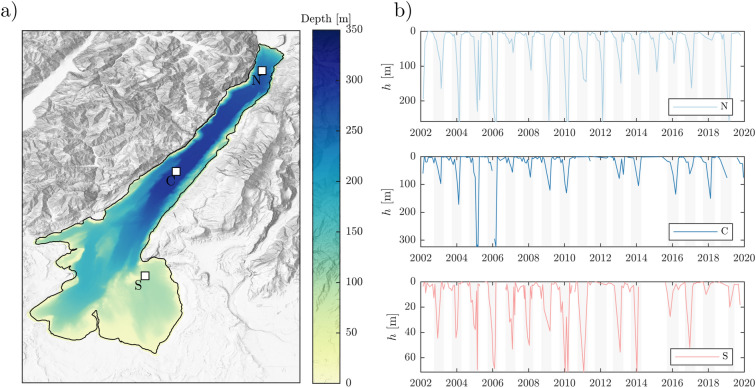
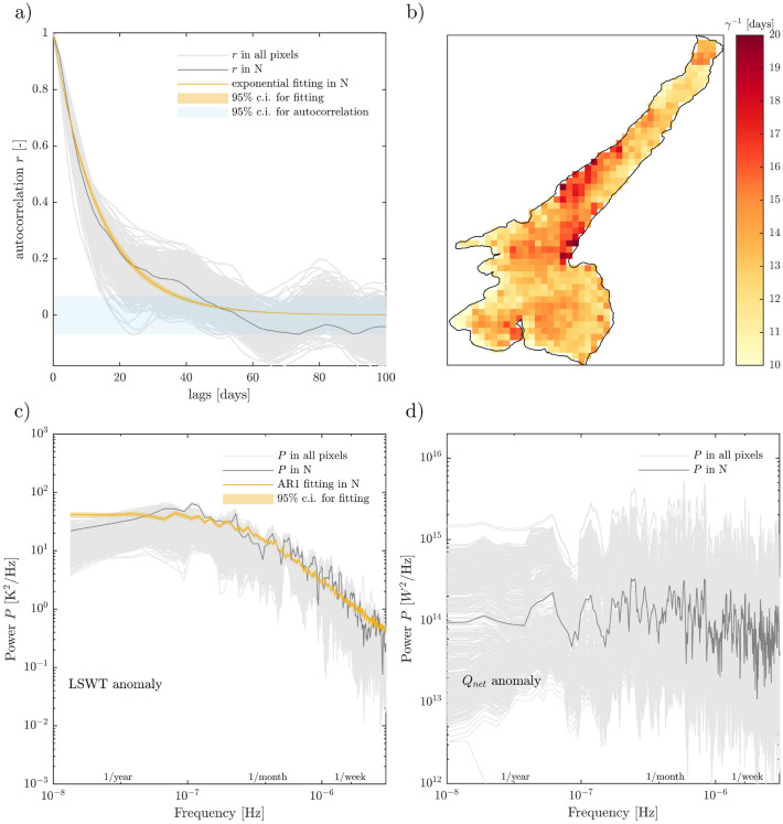
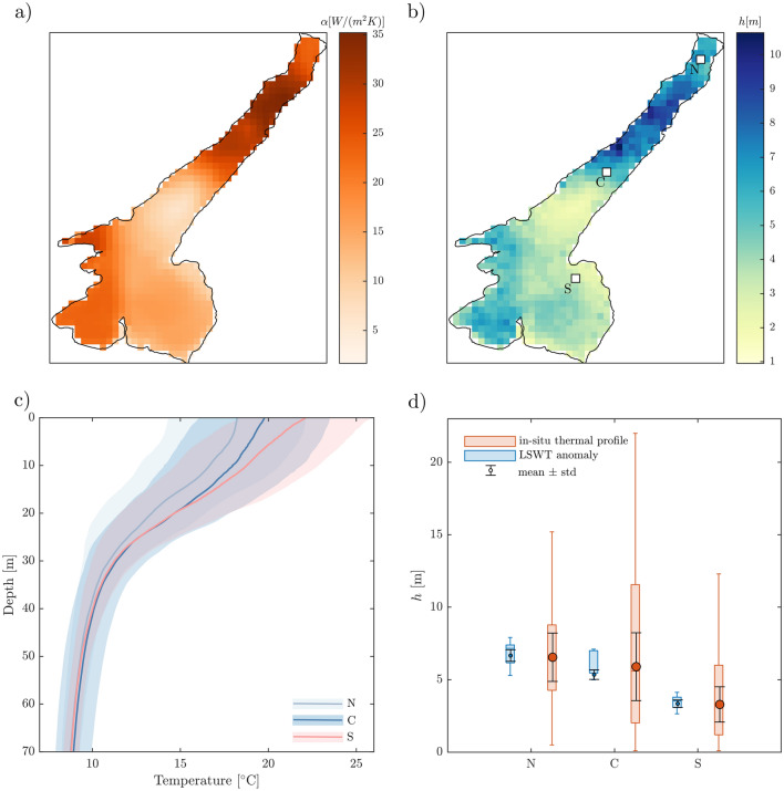
Slow and long-term variations of sea surface temperature anomalies have been interpreted as a red-noise response of the ocean surface mixed layer to fast and random atmospheric perturbations. How fast the atmospheric noise is damped depends on the mixed layer depth. In this work we apply this theory to determine the relevant spatial and temporal scales of surface layer thermal inertia in lakes. We fit a first order auto-regressive model to the satellite-derived Lake Surface Water Temperature (LSWT) anomalies in Lake Garda, Italy. The fit provides a time scale, from which we determine the mixed layer depth. The obtained result shows a clear spatial pattern resembling the morphological features of the lake, with larger values (7.18± 0.3 m) in the deeper northwestern basin, and smaller values (3.18 ± 0.24 m) in the southern shallower basin. Such variations are confirmed by in-situ measurements in three monitoring points in the lake and connect to the first Empirical Orthogonal Function of satellite-derived LSWT and chlorophyll-a concentration. Evidence from our case study open a new perspective for interpreting lake-atmosphere interactions and confirm that remotely sensed variables, typically associated with properties of the surface layers, also carry information on the relevant spatial and temporal scales of mixed-layer processes.

Figure 1

(a) Map of Lake Garda with location of in-situ monitoring points (white squares), bathymetry from the latest (2022) high resolution survey from the Hydrographic Institute of the Italian Navy (IIM), and orography of the surrounding region (topographic map credits: ESRItopo). The map shows how the northern part of the lake is flanked by steep slopes. (b) Mixed layer depth h estimated from in-situ monthly thermal profiles located as in (a). Light grey boxes indicate unstratified conditions, i.e, the months when temperature gradients between surface and deeper layers are below 1 ^∘C. Further information on the climatology of mixed layer depth in the monitoring points is provided in the Supplementary Material).

Figure 2

(a) Auto-correlation of LSWT anomaly at N (thick grey line, see Fig. 1 for the location) and in all other pixels (thin grey lines). Exponential fitting of r at N (orange line) and corresponding 95$\%$ confidence bounds (orange shadowed area). The horizontal light blue box shows the 95$\%$ confidence bounds considered for the computation of auto-correlation. (b) Spatial variability of the damping time scale (inverse of $\gamma$) obtained from exponential fitting in each pixel of the map. (c) Power spectra of LSWT anomalies in N (thick grey line) and in all other pixels (thin grey lines). Spectrum of a synthetic AR1 process computed at N (orange line) by considering $\gamma =0.0725d^{-1}$ ($\sim$ 14 days) and 95$\%$ confidence bounds (orange shadowed area) from 100 realisations. (d) White spectrum of net heat flux anomalies based on Delft3D model simulations on Lake Garda in all model pixels (thin grey lines) and in N (thick grey line).

Figure 3

(a) Spatial variability of the coefficient $\alpha$ based on linear regression of $Q_{\mathit{net}}$ anomaly as a function of $T_a-T_w$ anomaly in each grid cell of Delft3D model simulations on Lake Garda; (b) spatial variability of h estimated by inverting Eq. (3). The white squares identify the pixels closest to in-situ monitoring points and considered for panel (d); (c) Water temperature profiles at the three monitoring stations during the stratified months (from May to September). Shaded area shows the standard deviation and the line the average over the period 2002–2020; (d) Estimation of mixed layer depth h from LSWT anomaly (blue boxes) and in-situ measurements (orange boxes) at the three monitoring points. Blue boxes represent the spatial variability within a 3 by 3 pixels area of h as estimated by inverting Eq. (3) with $\gamma$ from Fig. 2. Orange boxes represent the temporal variability of h as computed from the timeseries of temperature profiles (2002–2020) assuming a threshold temperature between surface and interior layer of 0.1^∘. The median, the lower and upper quartiles of both estimates are shown as the orange/blue line inside the box, the bottom and top edges of the box respectively. The whiskers endpoints show the shallowest and deepest h from the sample. Errorbars overlapped on boxes show the uncertainty associated with the computation method: 95% confidence interval from the fitting of $\gamma$ for blue boxes; use of different threshold temperature gradient (from 0.1 to 1 ^∘C) for orange boxes.

Figure 4

Spatial distribution of temporal mean (top, a–c) and standard deviation (bottom, d–f) of LSWT (a,d), chl-a (b,e) and turbidity (c,f) in Lake Garda. Mean and standard deviations are computed on the gap-filled time series from 2007 to 2020 for LSWT (2 days timestep), and from 2003 to 2012 for chl-a and turbidity (10 days timestep).

Figure 5

Correlation (top) and variance (bottom) associated with the first dominant EOF of LSWT (a,d), chl-a (b,e) and turbidity (c,f) anomalies in Lake Garda.

References

1. Bouffard D, Wüest A. Convection in lakes. Annu. Rev. Fluid Mech. 2019;51:189–215. doi: 10.1146/annurev-fluid-010518-040506. - DOI
1. Kirillin G, Shatwell T. Generalized scaling of seasonal thermal stratification in lakes. Earth Sci. Rev. 2016;161:179–190. doi: 10.1016/j.earscirev.2016.08.008. - DOI
1. Gray E, Mackay EB, Elliott JA, Folkard AM, Jones ID. Wide-spread inconsistency in estimation of lake mixed depth impacts interpretation of limnological processes. Water Res. 2020;168:115136. doi: 10.1016/j.watres.2019.115136. - DOI - PubMed
1. Wilson HL, et al. Variability in epilimnion depth estimations in lakes. Hydrol. Earth Syst. Sci. 2020;24:5559–5577. doi: 10.5194/hess-24-5559-2020. - DOI
1. Wells, M. G. & Troy, C. D. Surface mixed layers in lakes. In Encyclopedia of Inland Waters, 2nd edn (eds. Mehner, T. & Tockner, K.) 546–561. (Elsevier, 2022). 10.1016/B978-0-12-819166-8.00126-2.