Extraction of persistent lagrangian coherent structures for the pollutant transport prediction in the Bay of Bengal

Abstract

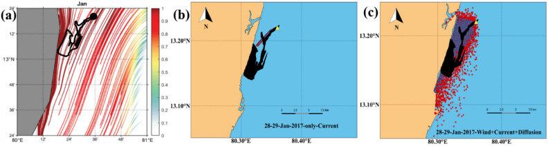
Lagrangian Coherent Structures (LCS) are the hidden fluid flow skeletons that provide meaningful information about the Lagrangian circulation. In this study, we computed the monthly climatological LCSs (cLCS) maps utilizing 24 years (1994-2017) of HYbrid Coordinate Ocean Model (HYCOM) currents and ECMWF re-analysis winds in the Bay of Bengal (BoB). The seasonal reversal of winds and associated reversal of currents makes the BoB dynamic. Therefore, we primarily aim to reveal the cLCSs associated with seasonal monsoon currents and mesoscale (eddies) processes over BoB. The simulated cLCS were augmented with the complex empirical orthogonal functions to confirm the dominant lagrangian transport pattern features better. The constructed cLCS patterns show a seasonal accumulation zone and the transport pattern of freshwater plumes along the coastal region of the BoB. We further validated with the satellite imagery of real-time oil spill dispersion and modelled oil spill trajectories that match well with the LCS patterns. In addition, the application of cLCSs to study the transport of hypothetical oil spills occurring at one of the active oil exploration sites (Krishna-Godavari basin) was described. Thus, demonstrated the accumulation zones in the BoB and confirmed that the persistent monthly cLCS maps are reasonably performing well for the trajectory prediction of pollutants such as oil spills. These maps will help to initiate mitigation measures in case of any occurrence of oil spills in the future.

Keywords: Accumulation; Bay of Bengal; Eddies; HYCOM; LCS; Pollutants; Prediction; Trajectory.

Figure 1

The constructed monthly cLCS maps during the Indian Summer Monsoon (SM) season over the Bay of Bengal. (a) June, (b) July, (c) August, (d) September. The colour bar in the figure represents the variation of climatological attraction strengths in lncρ, and the overlaid black arrow indicates the EICC direction in general during the SW monsoon period.

Figure 2

The constructed monthly cLCS maps during the Indian Winter Monsoon (WM) season over the Bay of Bengal. (a) November (b) December (c) January (d) February. (The colour bar in the figure represents the variation of climatological attraction strengths in lncρ). The overlaid black arrow in Fig (a),(b) indicates the EICC direction. The clockwise pattern of black arrows in Fig. (d) Indicates the anticyclonic eddy.

Figure 3

(a) Climatological LCSs for the November month (The colour bar in the figure represents the variation of climatological attraction strengths in lncρ) (b) November Climatological SSS (Sea Surface Salinity) over the Bay of Bengal for the period of 2015-present. Block rectangular box indicates the southward advection of freshwater plume primarily driven by the EICC. The corresponding strong cLCSs are also evident in this region, marked in a black rectangular box (Fig. (a)).

Figure 4

The constructed cLCSs maps during Pre and post-monsoon seasons, (a) October (post-monsoon), (b) March, (c) April, (d) May (Pre-monsoon). (The colour bar in the figure represents the variation of climatological attraction strengths in lncρ). The black arrow indicates the strong, attractive cLCSs corresponding to the anticyclonic eddy.

Figure 5

March climatological LCSs (The colour bar in the figure represents the variation of climatological attraction strengths in lncρ) (b) March climatological Sea level anomaly over BoB for 1994–2017. The square box inside Fig. 5a represents the strong cLCS induced by an anticyclonic eddy near Visakhapatnam, and Fig. 5b represents the presence of an anticyclonic eddy.

Figure 6

cLCS (a–f)(The colour bar in the figure represents the variation of climatological attraction strengths in lncρ) and complex EOF analysis mode-1 (g-l) and 2 (m-r) over the Bay of Bengal during 1994–2017 for the months of June, July, August, September, October and November.

Figure 7

cLCS (a–f) (The colour bar in the figure represents the variation of climatological attraction strengths in lncρ) and complex EOF analysis mode 1 (g–l) and 2 (m–r) over the Bay of Bengal during 1994–2017 for December, January, February, March, April and May.

Figure 8

(a) The basin-wide cLCS pattern over the Bay of Bengal during January and (b) Subset indicate the spill incident area, the zoomed view of square box in Fig. (a). (The colour bar in the figure represents the variation of climatological attraction strengths in lncρ).

Figure 9

(a). Climatological LCSs (The colour bar in the figure represents the variation of climatological attraction strengths in lncρ) for January overlaid with Sentinel-1 shape file image (black colour dot indicates spill location and a black shape file for spill spreading). (b) GNOME oil spill model trajectory (purple line) simulated with only currents overlay with the SAR observed oil slick shapefile (solid black). (c). GNOME oil spill model trajectory (red dots) simulated with winds, currents, and diffusion coefficient overlay with the SAR observed oil slick shapefile (solid black). The purple dots show the best guess.

Figure 10

(a) Distribution of oil spills along the East Coast of India (KG-Basin) in 2017, (b) Oil spill shapefile image on October 15, 2017 (ID No. AE71).

Figure 11

Observed monthly climatological (1994–2017) cLCS (The colour bar in the figure represents the variation of climatological attraction strengths in lncρ) patterns near KG-Basin overlaid by the mean current direction (black arrows demark flow pattern), and the dark circle show the hypothetical oil spill origin. Panels a, b, c and d represent the southwest monsoon, e, f, g, h, the northeast monsoon, and i, j, k, and l represent pre-monsoon seasons.

References

1. Mera D, Cotos JM, Varela-Pet J, Garcia-Pineda O. Adaptive thresholding algorithm based on SAR images and wind data to segment oil spills along the northwest coast of the Iberian Peninsula. Mar. Pollut. Bull. 2012;64:2090–2096. doi: 10.1016/j.marpolbul.2012.07.018. - DOI - PubMed
1. Ivshina IB, et al. Oil spill problems and sustainable response strategies through new technologies. Environ. Sci. Process Impacts. 2015;17(7):1201–1219. doi: 10.1039/C5EM00070J. - DOI - PubMed
1. Rajendran S, et al. Detection of Wakashio oil spill off Mauritius using Sentinel-1 and 2 data: Capability of sensors, image transformation methods, and mapping. Environ. Pollut. 2021;274:116618. doi: 10.1016/j.envpol.2021.116618. - DOI - PubMed
1. Gurumoorthi K, Suneel V, Trinadha Rao V, Thomas AP, Alex MJ. Fate of MV Wakashio oil spill off Mauritius coast through modelling and remote sensing observations. Mar. Pollut. Bull. 2021;172:112892. doi: 10.1016/j.marpolbul.2021.112892. - DOI - PubMed
1. Trinadha Rao V, Suneel V, Gurumoorthi MJ, Thomas AP. Assessment of MV Wakashio oil spill off Mauritius, Indian Ocean through satellite imagery: A case study. J. Earth Syst. Sci. 2022;131:21. doi: 10.1007/s12040-021-01763-3. - DOI