Practical Considerations and Limitations of Using Leaf and Canopy Temperature Measurements as a Stomatal Conductance Proxy: Sensitivity across Environmental Conditions, Scale, and Sample Size

Abstract

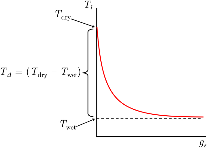
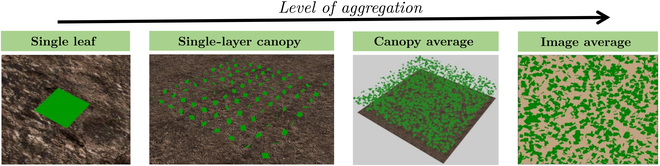
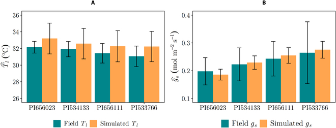
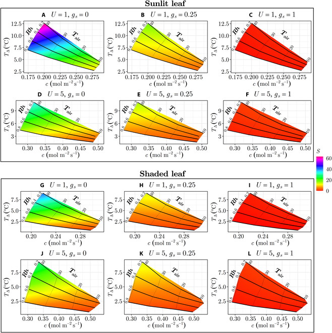
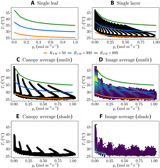
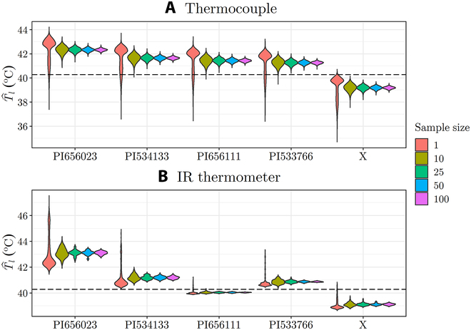
Stomatal conductance (g_s) is a crucial component of plant physiology, as it links plant productivity and water loss through transpiration. Estimating g_s indirectly through leaf temperature (T_l) measurement is common for reducing the high labor cost associated with direct g_s measurement. However, the relationship between observed T_l and g_s can be notably affected by local environmental conditions, canopy structure, measurement scale, sample size, and g_s itself. To better understand and quantify the variation in the relationship between T_l measurements to g_s, this study analyzed the sensitivity of T_l to g_s using a high-resolution three-dimensional model that resolves interactions between microclimate and canopy structure. The model was used to simulate the sensitivity of T_l to g_s across different environmental conditions, aggregation scales (point measurement, infrared thermometer, and thermographic image), and sample sizes. Results showed that leaf-level sensitivity of T_l to g_s was highest under conditions of high net radiation flux, high vapor pressure deficit, and low boundary layer conductance. The study findings also highlighted the trade-off between measurement scale and sample size to maximize sensitivity. Smaller scale measurements (e.g., thermocouple) provided maximal sensitivity because they allow for exclusion of shaded leaves and the ground, which have low sensitivity. However, large sample sizes (up to 50 to 75) may be needed to differentiate genotypes. Larger-scale measurements (e.g., thermal camera) reduced sample size requirements but include low-sensitivity elements in the measurement. This work provides a means of estimating leaf-level sensitivity and offers quantitative guidance for balancing scale and sample size issues.

Fig. 1.

Typical response of leaf temperature (T_l) to varying stomatal conductance (g_s). As g_s increases, the sensitivity of T_l to g_s (or slope of the curve) decreases. T_dry is the leaf temperature when g_s is 0, T_wet is the leaf temperature of an equivalent wet surface with unlimited supply of free water, and T_Δ is the difference between T_dry and T_wet.

Fig. 2.

Schematic diagram showing the different levels of aggregation used in simulated T_l measurement, scaling with an increase in the level of complexity from a single isolated leaf parallel to the ground, to a single-layer canopy of leaves randomly orientated with no self-shading, to a canopy average, and an image average representative of an aerial thermal image of the homogeneous canopy.

Fig. 3.

Field and simulated data for (A) T_l and (B) g_s averaged across each genotype. The simulated T_l and g_s are in an acceptable range with measured field data, which shows that the developed sorghum geometry can reliably produce acceptable simulations. The hat operator denotes a spatial average.

Fig. 4.

Variation in the sensitivity (S) of leaf temperature to stomatal conductance with changes in ambient conditions and stomatal conductance (g_s). Each subplot represents different combinations of relative humidity (Rh) ranging from 0.2 to 0.8 and air temperature (T_air) varying from 10 to 40^∘C. The columns correspond to different g_s ranging from 0 to 1  mol  m⁻²  s⁻¹. (A to F) Conditions for a sunlit leaf (R_SW = 300  W  m⁻²). (G to L) Shaded leaf (R_SW = 50  W  m⁻²). The wind speed (U) remains constant within each row, with (A) to (C) and (G) to (I) having U of 1  m  s⁻¹, and (D) to (F) and (J) to (L) having U of 5  m  s⁻¹. To interpret this plot, a subplot is selected based on ambient radiation level, wind speed, and expected stomatal conductance. The S value can be determined by matching the surface color at the given ambient air temperature and humidity to the associated value in the color bar.

Fig. 5.

Relationship between T_l and g_s for different levels of aggregation at constant ambient conditions of 30^∘C  (T_air), 0.5  (Rh), and 1  m  s⁻¹  (U). (A) Trend of an isolated single leaf with absorbed radiation flux R_SW of 50, 300, and 600 W  m⁻². The line plots of the single leaf were replotted in (B) to (D) to show how the single leaf T_l − g_s trend relates when scaling at a canopy level. Each spike shown in (B) (single layer), (C) (canopy average with sunlit leaves), and (D) (canopy average with shaded leaves) is a single E_m value, which was set in the stomatal conductance model to vary the g_s values. (D and F) Aerial thermal image (image average) of the homogeneous canopy for sunlit and shaded thermal pixels, respectively. The brighter yellow colors in (D) and (F) shows the highest density of thermal pixel data points.

Fig. 6.

The fraction of sunlit leaves (f_sun) with varying LAI is shown for (A) canopy average and (B) image average, which also includes how much of the ground is viewed in a thermal image (f_ground) for different LAI (f_ground does not change with solar zenith angle). Variation in average S with varying g_s, LAI, solar zenith, and aggregation scale is shown in (C) to (I): (C) single-layer canopy, (D) canopy average with LAI = 0.5, (E) canopy average with LAI = 1.5, (F) canopy average with LAI = 3, (G) image average with LAI = 0.5, (H) image average with LAI = 1.5, and (I) image average with LAI = 3. The single layer generally has the highest S because there are no shaded leaves. For the canopy averages, S decreases with an increase in LAI due to the increase in the fraction of shaded leaves. For the image averages, S increases with an increase in LAI due to the decrease in ground exposure. The hat operator denotes a spatial average.

Fig. 7.

(A) Visualization of 3D model sorghum canopy. (B) Example of simulated aerial thermal images captured by the thermal camera for five sorghum genotypes under conditions of high S (favorable) and low S (unfavorable). Images show the difference between surface temperature and ambient air temperature (T_air = 40.3^∘C for favorable, and T_air = 14.1^∘C for unfavorable) in order to increase contrast.

Fig. 8.

Ability of the thermal camera to detect a difference in average stomatal conductance among sorghum genotypes for varying camera viewing angles and environmental conditions. (A) to (C) compare different viewing angles at environmental conditions with moderate sensitivity: (A) 0^∘, (B) 15^∘, and (C) 30^∘ between the thermal camera viewing direct and sun direction. (D) Results for a viewing direction of 0^∘, but unfavorable conditions. Error bars indicate standard deviation. Groups sharing the same letter are not statistically different from each other at a significance level of α= 0.05, based on Dunn’s post hoc analysis following Kruskal–Wallis test. S had the same significance designations as T_l, and g_s is significantly different across genotypes for all cases. The hat operator denotes a spatial average.

Fig. 9.

Violin plots showing the T_l distribution across genotypes for (A) thermocouple and (B) IR thermometer conducted under favorable conditions (T_air = 40.3^∘C, Rh = 0.18, U = 2.77 m s⁻¹). gs of the genotypes decreases from left to right, and the horizontal dotted lines represent the air temperature. The hat operator on ${\widehat{T}}_l$ denotes that average values of T_l were considered in this scenario.

References

1. Brodribb TJ, Holbrook MA, Zwieniecki NM, Palma B.. Leaf hydraulic capacity in ferns, conifers and angiosperms: Impacts on photosynthetic maxima. New Phytol. 2005;165(3):839–846. - PubMed
1. Buckley TN. How do stomata respond to water status? New Phytol. 2019;224(1):21–36. - PubMed
1. Sinclair TR, Tanner CB, Bennett JM. Water-use efficiency in crop production. Bioscience. 1984;34(1):36–40.
1. Messina CD, Sinclair TR, Hammer GL, Curan D, Thompson J, Oler Z, Gho C, Cooper M. Limited-transpiration trait may increase maize drought tolerance in the us corn belt. Agron. J. 2015;107(6):1978–1986.
1. Raymundo R, Mclean G, Sexton-Bowser S, Morris GP. Crop modeling suggests limited transpiration would increase yield of sorghum across drought-prone regions of the United States. bioRxiv. 2023. 10.1101/2023.06.27.546776. - DOI - PMC - PubMed