Deep learning methods in metagenomics: a review

Abstract

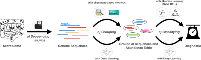
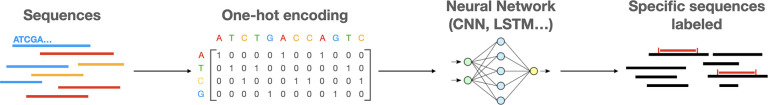
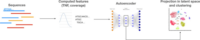
The ever-decreasing cost of sequencing and the growing potential applications of metagenomics have led to an unprecedented surge in data generation. One of the most prevalent applications of metagenomics is the study of microbial environments, such as the human gut. The gut microbiome plays a crucial role in human health, providing vital information for patient diagnosis and prognosis. However, analysing metagenomic data remains challenging due to several factors, including reference catalogues, sparsity and compositionality. Deep learning (DL) enables novel and promising approaches that complement state-of-the-art microbiome pipelines. DL-based methods can address almost all aspects of microbiome analysis, including novel pathogen detection, sequence classification, patient stratification and disease prediction. Beyond generating predictive models, a key aspect of these methods is also their interpretability. This article reviews DL approaches in metagenomics, including convolutional networks, autoencoders and attention-based models. These methods aggregate contextualized data and pave the way for improved patient care and a better understanding of the microbiome's key role in our health.

Keywords: binning; deep learning; disease prediction; embedding; metagenomics; microbiome; neural network.

Fig. 1.. Illustration of the use of deep learning in disease prediction from metagenomic data. The classic simplified pipeline for disease prediction from microbiome data follows three distinct steps. In step (a), high-throughput sequencing of DNA libraries from samples generates millions of reads (from whole genomic DNA in WGS metagenomics or from targeted 16S rRNA genes in targeted metagenomics) from the organisms that make up the community. Second, in step (b), the sequences are either clustered or classified into different groups to characterize the different species present in the sample. This step can be realized by classical bioinformatics pipelines, such as alignment-based methods, or by more recent DL architectures, both of which can be used to estimate their relative abundance. In step (c), the abundance table or the embeddings extracted from the use of neural networks can be used to classify the metagenomes as coming from patients with the disease state or not. DL methods can also be used to integrate additional information (annotations, genes, phylogeny) to classify sequences or metagenome profiles.

Fig. 2.. Article selection methodology used in this paper. (a) The pipeline of our methodology for choosing articles. It consists of three steps. (A) Articles are extracted from three databases using our research equation. (B) Remaining articles are provided as anchors to Connected Papers, which generates similarity graphs for each article. Once retrieved, the graphs are integrated in a unified graph. Articles with a certain number (that we will set to 4) of links pointing towards them are added to the selection. (C) The newly added articles are filtered using the same research equation as in step (A), but searching words in keywords and abstract instead of title. Numbers correspond to the second phase of screening. (b) PRISMA-type diagram for article selection of this review. The method developed here enriches the research equation selection with Connected Papers; this diagram represents the selection along with this enrichment in green.

Fig. 3.. Sequence mining workflow diagram. DNA sequences are encoded, most of the time with one-hot encoding, which leaves a matrix of dimensions 4 by the length of the sequence. The sequence is then analysed by a neural network, often a CNN, to be classified as a specific type of gene, for instance a viral sequence. Adapted from: [83].

Fig. 4.. Example of an unsupervised binning method using autoencoder. Features like TNF (tetranucleotide frequency) or coverage are extracted from sequences and analysed by an autoencoder, to create an embedding vector representing the sequence. This vector is then projected in a latent space, allowing visualization and clustering of sequences. Adapted from [118].

Fig. 5.. Classification with sequence embedding MIL pipelines This pipeline is shared by both Metagenome2Vec [125] and IDMIL [57]. The arrows above correspond to IDMIL, the lower ones to Metagenome2Vec. Step (a) presents how sequences are embedded: their k-mers are extracted and embedded using NLP methods. These embedded k-mers are then used to obtain the embedding of a read, whether through their mean or by learning the relationship between k-mer embeddings and read embeddings through DL. Step (b) presents how these embedded reads are grouped together. IDMIL uses unsupervised clustering with k-means, while Metagenome2Vec groups reads by genomes. Both obtain groups of read embeddings, which must then be embedded themselves. Here, IDMIL chooses a read representative for each group, while Metagenome2Vec chooses the mean. These group embeddings represent the metagenome differently: the first method orders them in a matrix and uses a CNN for prediction while Metagenome2Vec treats them like a bag of instances and uses MIL methods such as DeepSets [152] to analyse them.

Fig. 6.. Taxonomy-aware metagenome classification method, as performed with PopPhy-CNN. Phylogeny between taxa is used to create a tree, and abundance to populate it. This tree is then embedded as a matrix used as input for a CNN that will ultimately classify the metagenome. Modified from [157].

Fig. 7.. Overview of different steps and methods in disease prediction from metagenomic data. These steps represent the entire pipeline from raw reads to disease prediction. Note that not all steps are required and some methods described in a step are not always compatible with every method from the next step. This figure aims to represent the diversity of method in each step, not necessarily every entire pipeline possible. Moreover, as previously stated, most methods only perform half of the steps: the first half from reads or contigs (steps Input or Assembly) to their classification (steps Result or Metagenome Representation) and the second half for disease prediction (step Metagenome Representation to Output). Input represents the raw sequences acquired through sequencing. Assembly can either be the long or short reads acquired previously, or the contigs assembled from these reads. Representations are the way these features will be fed to the DL model (encoding, features). DL Method for Sequences show the different types of networks used to extract features. Results are the output of these networks: classification, clustering and embedding, which can then be used for Metagenome Representation, along with other sources. These representations are then filtered or transformed through Data processing, resulting in Processed data (images, tables, clusters). DL method for Metagenome are then used to treat these features and produce an Output: diagnosis, data visualization, phenotype evolution.

References

1. Marchesi JR, Ravel J. The vocabulary of microbiome research: a proposal. Microbiome. 2015;3:31. doi: 10.1186/s40168-015-0094-5. - DOI - PMC - PubMed
1. Sunagawa S, Coelho LP, Chaffron S, Kultima JR, Labadie K, et al. Ocean plankton. Structure and function of the global ocean microbiome. Science. 2015;348:1261359. doi: 10.1126/science.1261359. - DOI - PubMed
1. Bahram M, Hildebrand F, Forslund SK, Anderson JL, Soudzilovskaia NA, et al. Structure and function of the global topsoil microbiome. Nature. 2018;560:233–237. doi: 10.1038/s41586-018-0386-6. - DOI - PubMed
1. Consortium HMP. Structure, function and diversity of the healthy human microbiome. Nature. 2012;486:207–214. doi: 10.1038/nature11234. - DOI - PMC - PubMed
1. Zimmerman S, Tierney BT, Patel CJ, Kostic AD. Quantifying shared and unique gene content across 17 microbial ecosystems. mSystems. 2023;8:e0011823. doi: 10.1128/msystems.00118-23. - DOI - PMC - PubMed
LinkOut - more resources