Control of working memory by phase-amplitude coupling of human hippocampal neurons

Abstract

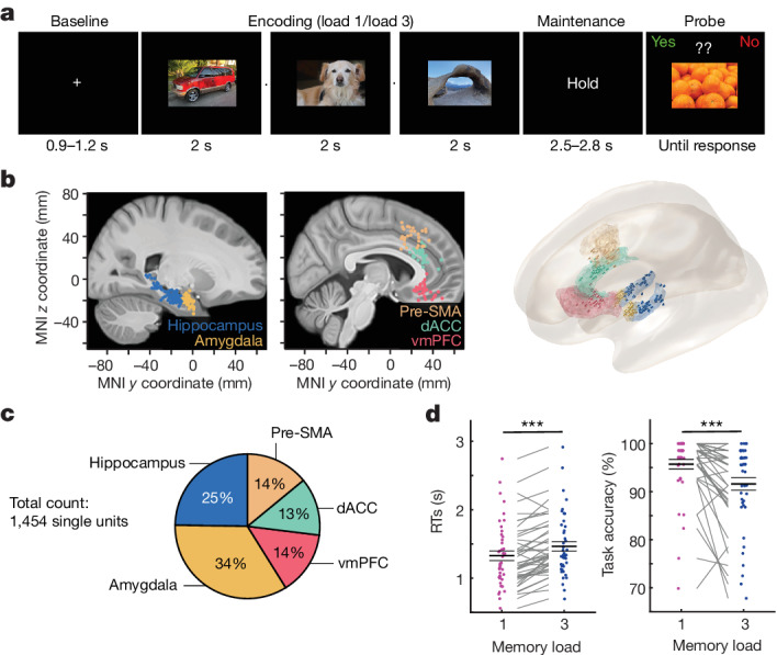
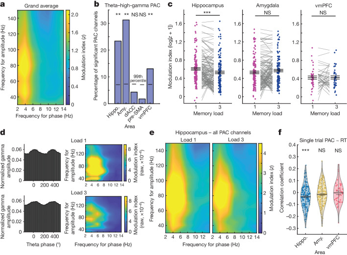
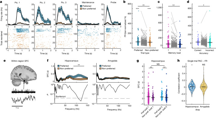
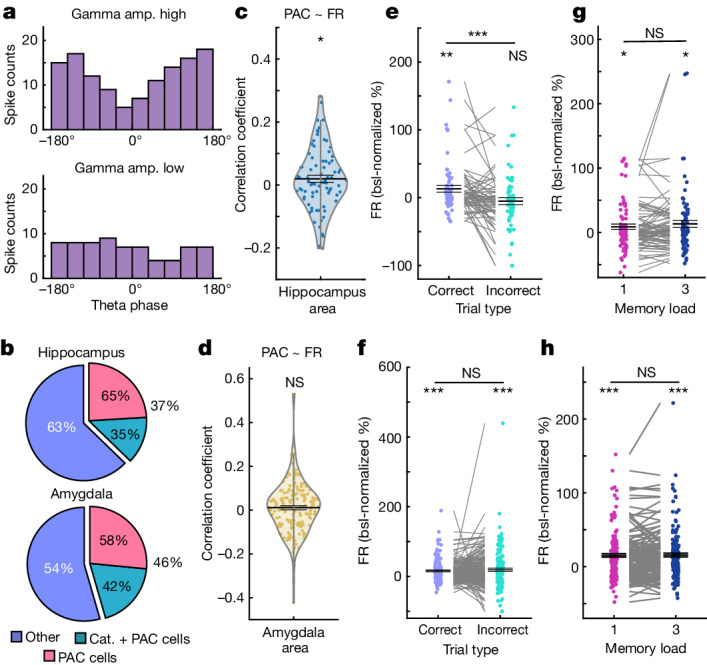
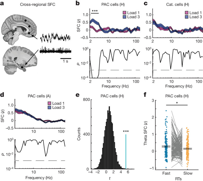
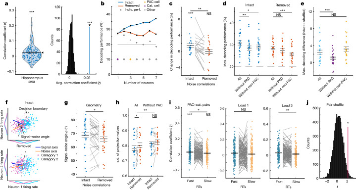
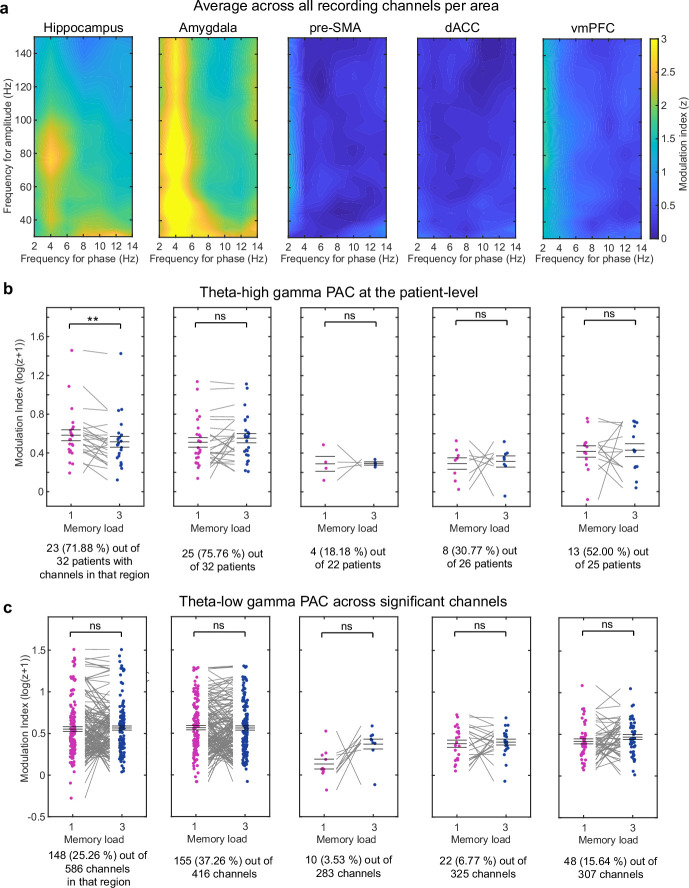
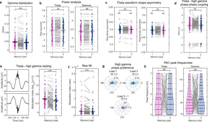
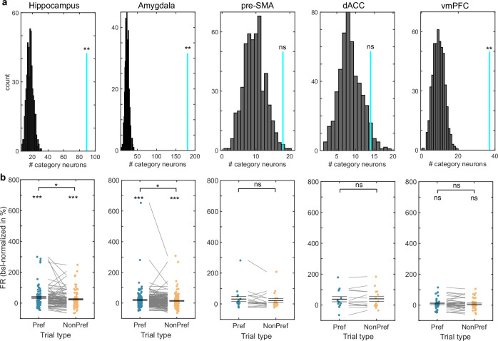
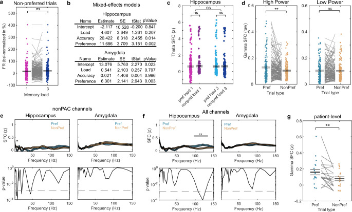
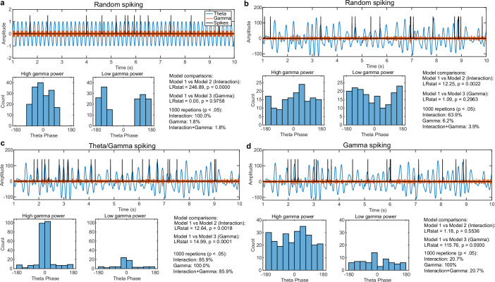
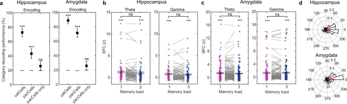
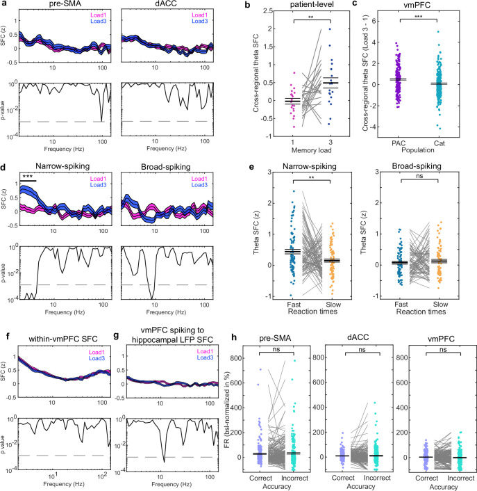
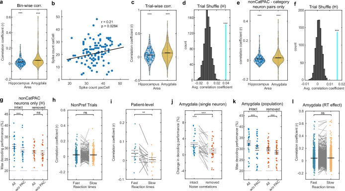
Retaining information in working memory is a demanding process that relies on cognitive control to protect memoranda-specific persistent activity from interference^1,2. However, how cognitive control regulates working memory storage is unclear. Here we show that interactions of frontal control and hippocampal persistent activity are coordinated by theta-gamma phase-amplitude coupling (TG-PAC). We recorded single neurons in the human medial temporal and frontal lobe while patients maintained multiple items in their working memory. In the hippocampus, TG-PAC was indicative of working memory load and quality. We identified cells that selectively spiked during nonlinear interactions of theta phase and gamma amplitude. The spike timing of these PAC neurons was coordinated with frontal theta activity when cognitive control demand was high. By introducing noise correlations with persistently active neurons in the hippocampus, PAC neurons shaped the geometry of the population code. This led to higher-fidelity representations of working memory content that were associated with improved behaviour. Our results support a multicomponent architecture of working memory^1,2, with frontal control managing maintenance of working memory content in storage-related areas^3-5. Within this framework, hippocampal TG-PAC integrates cognitive control and working memory storage across brain areas, thereby suggesting a potential mechanism for top-down control over sensory-driven processes.

Fig. 1. Task, recording sites and behaviour.

a, An example trial. Each trial consisted of either one (load 1) and three (load 3) consecutively presented pictures, each presented for 2 s (separated by a variable blank screen of up to 200 ms as indicated by a small dot). After a variable maintenance period with an average duration of 2.7 s, a probe picture was presented. The task was to decide whether the probe picture has been part of the pictures shown during encoding in this trial (the correct answer was ‘No’ in the example shown). For copyright reasons, the pictures shown are similar but not identical to those used in the study. b, The recording locations. Each coloured dot represents the location of a microwire bundle across all 44 sessions shown on a standardized MNI152 brain template (left) and in a 3D model using the Brainnetome Atlas (right). The slices (https://osf.io/r2hvk/) were obtained under a Creative Commons licence CC BY 4.0. c, The proportions of neurons recorded in each brain area. d, The behaviour of the participants. Patients made fewer errors (P = 0.0001) and responded faster (P = 0.0001) in load 1 compared with load 3 trials. Statistical analysis was performed using two-sided permutation-based t-tests with 10,000 permutations. Each line connects the two dots belonging to the same session. n = 44 sessions. The RT was measured relative to the probe stimulus onset. Data are mean ± s.e.m. ***P < 0.001.

Fig. 2. TG-PAC.

a, Average normalized modulation indices for all phase–amplitude pairs. n = 1,917 channels. b, The proportion of channels with significant theta–high-gamma PAC in each area, determined by comparisons to trial-shuffled surrogates (both loads). The horizontal lines indicate the 99th percentile of the surrogate null distribution per area (P = 0.005 for hippocampus (hippo.), amygdala (amy.) and vmPFC; right-sided permutation test, no adjustment for multiple comparisons). c, log-normalized modulation indices were averaged within the theta–high-gamma band in each load and compared between the loads in each significant PAC channel in each region. Only in the hippocampus, theta–high-gamma PAC differed as a function of load, with PAC higher in load 1 versus load 3 trials (left: n = 137 channels, P = 0.0005; amygdala (middle): n = 130, P = 0.38; vmPFC (right): n = 40, P = 0.87; two-sided permutation-based t-tests; FDR corrected for all five brain areas). z-scored values were shifted into a positive range by an offset of 1 and log-transformed for illustrative purposes only. All statistics are based on non-transformed z values. d, Example gamma amplitude distribution over theta phase as well as comodulograms with raw modulation indices in each load for a representative hippocampal channel. Note the wider distribution of gamma amplitude over theta phase in load 3 trials, which leads to lower levels of PAC (further analysis is provided in Extended Data Fig. 3a). Normalized MI values were as follows for the two examples shown: load 1, z = 16.52; load 3, z = 7.92. e, Average normalized modulation indices for significant hippocampal PAC channels. n = 137. f, TG-PAC was significantly negatively correlated with RTs in the hippocampus (n = 137, P = 6 × 10⁻⁵, mixed-effects GLM), but not in the amygdala (n = 130, P = 0.48) or the vmPFC (n = 40, P = 0.24). GLM results are shown in Supplementary Table 2. Each dot represents a significant PAC channel. For c,f, data are mean ± s.e.m. *P < 0.05; NS, not significant.

Fig. 3. FRs and SFC of category neurons in MTL.

a, Example hippocampal category neuron. The preferred category of this neuron was ‘animals’. Pic., picture. b, Category neurons (n = 270) remained active (preferred (pref.) versus baseline (bsl), P = 0.0001; non-preferred (non-pref.), P = 0.0001) and retained their selectivity during the maintenance period, with FRs higher for preferred compared with non-preferred categories (P = 0.001). FRs are shown as the percentage change compared with the baseline (−0.9 to −0.3 s before picture 1 onset). c, FRs of category neurons were higher in load 1 compared with load 3 trials with their preferred category held in WM (n = 270, P = 0.004) during the maintenance period. d, Category neurons fired more in correct compared with incorrect trials (n = 246, P = 0.02). e, SFC between spikes and LFPs from the same area. The slice (https://osf.io/r2hvk/) was obtained under a Creative Commons licence CC BY 4.0. f, Paired with PAC channels, hippocampal category neurons were more strongly phase-locked to local gamma LFPs with the preferred category held in WM (n = 151 combinations; P = 0.004). Differences were not significant in the amygdala (n = 423) or non-PAC channels (Extended Data Fig. 5e). Statistical analysis was performed using two-sided cluster-based permutation t-tests. g, Gamma (70–140 Hz) SFC for hippocampal category neurons was stronger for preferred versus non-preferred trials in both load conditions (main effect preference, F_1,150 = 16.23, P = 0.0001; load 1, P = 0.003; load 3, P = 0.004). No main effect of load (P = 0.25) or interaction (P = 0.33) was found. Each dot is a neuron–LFP channel pair (n = 151). h, TG-PAC was positively correlated with the FR of category neurons in the hippocampus (n = 151, P = 0.017, mixed-effects GLM), but not in the amygdala (n = 423, P = 0.45). The GLM results are shown in Supplementary Table 3. For b–d,g, statistical analysis was performed using two-sided permutation-based t-tests (b–d, lower brackets in g) and F-tests (top bracket in g). For a–d,f–h, data are mean ± s.e.m. (coloured areas in a,f); **P < 0.01.

Fig. 4. PAC neuron selection and local activity.

a, The binning used for PAC neuron selection for an example hippocampal neuron. Theta phase, binned into ten groups, and gamma amplitude (amp.), median split into low and high, were used to predict the spike counts of each neuron from the MTL during the delay. The spike count was higher during high-gamma amplitudes (gamma main effect) and differed in their theta phase distribution between high and low gamma amplitudes (interaction effect), resulting in selecting this neuron as a PAC neuron. b, The proportions of neurons qualifying as PAC neurons. Cat., category. c,d, FRs of PAC neurons were positively correlated with single-trial estimates of TG-PAC in the hippocampus (c; n = 79, P = 0.028, mixed-effects GLM), but not in the amygdala (d; n = 163, P = 0.98; GLM results are shown in Supplementary Table 4). e,f, FRs of PAC neurons during the maintenance period differed between correct and incorrect trials in the hippocampus (e; n = 63; correct versus baseline, P = 0.01; incorrect, P = 0.33; correct − incorrect, P = 0.0001; 16 neurons were excluded due to insufficient data in the incorrect condition), but not in the amygdala (f; n = 156; correct, P = 0.0001; incorrect, P = 0.0001; correct − incorrect, P = 0.45; 7 were neurons excluded due to insufficient data in the incorrect condition). FRs are shown as the percentage change compared with the baseline (−0.9 to −0.3 s). g,h, FRs did not differ between loads (hippocampus (g): n = 79; load 1, P = 0.03; load 3, P = 0.01; load 3 − load 1, P = 0.20; amygdala (h): n = 163; load 1, P = 0.0001; load 3, P = 0.0001; load 3 − load 1, P = 0.80). For g–j, statistical analysis was performed using two-sided permutation-based t-tests. For e–j, data are mean ± s.e.m.

Fig. 5. Remote connectivity of PAC neurons in the MTL to frontal theta LFPs.

a, Long-range SFC between MTL spiking activity and LFPs recorded from all three frontal regions. The slices (https://osf.io/r2hvk/) were obtained under a Creative Commons licence CC BY 4.0. b, Spikes of hippocampal PAC neurons were more strongly synchronized with theta-band LFPs recorded in the vmPFC during the maintenance period during load 3 compared with load 1 trials (n = 175 connections; cluster P = 0.0001). This was not the case for the pre-SMA and dACC (Extended Data Fig. 8). c,d, Category neurons from the hippocampus (c; n = 215) or PAC neurons from the amygdala (d; n = 767) did not show significant SFC differences between loads relative to the vmPFC LFP. For b–d, statistical analysis was performed using two-sided cluster-based permutation t-tests with a Bonferroni-corrected alpha-level for two MTL areas, three frontal areas and two cell populations. e, Hippocampal PAC cells (n = 175, cyan line) yielded the strongest long-range theta SFC difference between load 3 and load 1 trials among 10,000 random selections of hippocampus–vmPFC connections (P = 0.0001, right-sided permutation test). t values correspond to comparisons between load 3 and load 1 trials for an average of SFC values in the significant theta range (2.5–4.3 Hz). For b–d, data are mean (centre line) ± s.e.m. (coloured areas). f, The remote theta-band SFC between spiking activity of PAC neurons and LFPs recorded in the vmPFC was significantly stronger for fast compared with slow RT trials (P = 0.03, two-sided permutation-based t-test). Each dot is a neuron-channel connection (n = 167; 8 connections were excluded due to inefficient spike count in at least one of the conditions). Data are mean ± s.e.m. A, amygdala; H, hippocampus.

Fig. 6. Noise correlations of PAC neurons in the hippocampus.

a, The mean correlation for all category–PAC neuron pairs was positive (n = 162, P = 0.0001) (left). Right, the mean correlation was larger than the null distribution of mean correlations without noise correlations (P = 0.001, right-sided permutation test). b, The decoding accuracy for category from FR in the maintenance period with intact or removed noise correlations for an example session. The white dots signify accuracy, and the coloured dots indicate the identity for each neuron. Indiv., individual. c, Adding single PAC neurons to the ensemble with intact noise correlations increased the decoding accuracy (n = 21; intact, P = 0.0007; removed, P = 0.91; intact − removed, P = 0.003). d, Removing PAC neurons reduced decodability with intact noise correlations only (n = 22 sessions; intact, P = 0.004; removed, P = 0.20). Removing non-PAC neurons decreased decoding for intact (P = 0.010) and removed (P = 0.0001) correlations. e, The decoding difference with and without noise correlations was lower only when PAC neurons were removed (n = 22 sessions; PAC, P = 0.0007; non-PAC, P = 0.10). f, The signal–noise axis for simulated tuned (neuron 1) and untuned (neuron 2) neurons. The signal–noise axis angle is reduced without noise correlations. g, The signal–noise angle in the data was reduced after removing noise correlations (n = 32 sessions, P = 0.009). h, The variance along the signal axis was reduced when noise correlations were intact only when PAC neurons were present (n = 19 sessions, P = 0.014; main effect ensemble: P = 0.0013; permutation-based F-test). i, Correlations of PAC–category pairs (n = 162) were stronger in fast (P = 0.0001) compared with slow (P = 0.06; median split; fast − slow, P = 0.028; preferred category trials only) RT trials. This effect was significant in load 3 (P = 0.009) but not in load 1 (P = 0.34) trials. j, The PAC–category pair correlation difference between fast and slow RT trials was larger than for random non-PAC–category pairs (P = 0.016, right-sided permutation test). For a,c–e,g–i, statistical analysis was performed using two-sided permutation-based t-tests. Data are mean ± s.e.m.

Extended Data Fig. 1. Spike-sorting quality metrics for all identified putative single units and wavelet characteristics.

(a-e) Spike-sorting quality metrics. (a) Proportion of inter-spike intervals (ISI) below 3 ms. (b) Average firing rate. (c) Coefficient-of-variation. (d) Signal-to-noise ratio (SNR) for the peak of the mean waveform across all spikes as compared to the standard deviation of the background noise. (e) Mean SNR of the waveform. (f) Example raw LFP recorded in a hippocampal channel during the delay period of a single trial (time 0 denotes onset of the delay period). (g) Power-spectrum of LFP data shown in (f). (h,i) Wavelet characteristics for all 40 wavelets used. Left: Wavelet family. The upper panel shows the temporal outline and the magnitude of the real part for all wavelets smoothed across all frequencies. The maximal magnitude of each wavelet is scaled to 1. Warm colours denote positive, cold colours negative magnitude. The lower panel shows the real part of all wavelets plotted on top of each other. Centre: The upper panel shows the spectral bandwidth of each wavelet as a function of centre frequency. The lower panel plots the FFT-spectrum for each wavelet. Right: The upper panel shows the temporal width of all wavelets as a function of centre frequency. The horizontal lines indicate the spectral bandwidth for each wavelet. The lower panel contains the amplitude envelope for each wavelet as a function of time. (j) Example original and reconstructed signal after applying the continuous wavelet transform (see Methods). Small deviations from the original signal are due to the fact that signals at frequencies lower or higher than the edge frequencies of 2 and 150 Hz, respectively, were not represented by the wavelet transform but present in the original signal. (k) Assessment of the wavelet-based signal reconstruction. We computed linear models using the reconstructed signal as predictor for the original signal and extracted R-squared values as a function of time and frequency in each trial and channel. Values were averaged across all trials and all hippocampal channels. An R-squared values of close to 1 indicates almost perfect reconstruction of the original signal. As stated above, the slight drop in reconstruction quality at extreme frequencies is explained by the fact that signals at frequencies lower or higher than the edge frequencies, respectively, were not represented by the wavelet transform but present in the original signal.

Extended Data Fig. 2. Additional PAC analyses.

(a) PAC comodulogram averaged across all channels separately for each area. Strongest PAC was observed between theta and gamma in both areas of the MTL. Frontal areas did not show strong PAC, with weak PAC at <2 Hz in pre-SMA and vmPFC. We focused our analysis on frequencies above 2 Hz (1–3 Hz bandpass) to ensure that at least 2 full cycles fit within our analysis window of 2.5 s (length of maintenance period). (b) In addition to testing theta-gamma PAC across significant channels (see main text), we tested PAC between the load conditions across patients after averaging all significant PAC channels within each patient. The results were similar to the analysis across channels, with strongest PAC in MTL areas and only weak PAC in frontal channels (see percent of patients with significant PAC channels below each figure), suggesting that the results were not driven by channels from a single patient. Only in the hippocampus again, PAC was stronger for load 1 as compared to load 3 (n = 23 patients, p = 0.0049), observable in almost each single patient. No significant differences were found between the load conditions in other regions (amygdala: n = 25; pre-SMA: n = 4; dACC: n = 8; vmPFC: n = 13). z-scored PAC values were shifted into a positive range by an offset of 1 and log-transformed for illustrative purposes only. All statistics are based on non-transformed z-values. (c) Theta to low gamma (30–55 Hz) PAC analyses. We also found strongest theta-low gamma PAC in MTL regions as opposed to frontal regions (see percentages below each figure). But for the low gamma band, we did not observe significant differences between the load conditions in any of the regions (hippocampus: n = 148 channels; amygdala: n = 155; pre-SMA: n = 10; dACC: n = 22; vmPFC: n = 48). See Supplementary Table 2 for additional PAC analysis separated into slow and fast theta. In (b,c), we performed two-sided permutation-based t-test and centre values denote mean ± s.e.m.; ** p < 0.01; ns = not significant.

Extended Data Fig. 3. Theta-high gamma PAC control analyses in the hippocampus.

(a) Higher memory loads are thought to be accompanied by a wider distribution of gamma amplitudes across theta phases, thereby leading to lower PAC values. To quantify the width of the distribution of gamma amplitude as a function of theta phase in load 3 than load 1, we estimated kappa. Kappa is a measure that describes the concentration (inverse of variance) of a circular variable around the mean direction. Across all PAC channels, kappa was significantly lower in load 3 compared to load 1 (n = 137 channels, t(136) = −3.7453, p = 0.0001) trials. This shows that gamma amplitudes are high for a wider range of theta phases for higher memory loads, thereby explaining why PAC decreases for higher memory loads. (b) Comparison of theta and gamma power. The significant hippocampal PAC channels showed no significant differences in theta or gamma power between the two load conditions (n = 137). (c) To determine the influence of theta waveform shape on PAC, we tested for differences in theta waveform peak-to-trough as well as rise-to-decay asymmetries between the two load conditions (see Methods). We did not find systematic differences between the conditions for both measures (n = 137). Moreover, average theta waveforms were overall symmetric as both measures were not significantly different from .5 in any of the conditions. (d) Moreover, if the differences between the load conditions observed for PAC channels in the hippocampus were explained by waveform shape differences/theta harmonics, we should also observe an effect for cross-frequency phase-phase coupling between the same frequency bands. We tested for that in all significant hippocampal PAC channels and did not observe a significant difference (n = 137). Theta-high gamma phase-phase coupling was computed as described in^,. (e) We determined the number of significant PAC channels that showed theta-high gamma nesting as described by Vaz et al. The left upper and lower panels show two examples of significant PAC channels from the hippocampus that were determined to have nesting by the Vaz et al. method (at least three local maxima within a window of 45 ms around the preferred phase (see Methods)). 110 of the 137 significant PAC channels (80.29%) in the hippocampus showed nesting between high gamma and theta. When testing PAC between the load conditions after removing channels that did not show significant nesting, PAC was still significantly lower in load 3 than 1 (n = 110; t(109) = −4.10; p = 0.0001). (f) Comparison of theta-gamma PAC strength in the hippocampus assessed using the raw modulation index rather than the of z-transformed MI. Raw theta-gamma PAC was significantly larger in load 1 compared to load 3 (n = 137; t(136) = −4.0264, p = 0.0001). (g) Distribution of theta phases at which gamma amplitude was maximal across all significant PAC channels in the hippocampus in load 1 and 3 (upper part). In most channels, gamma amplitude was maximal at the peak or the trough of theta. Note that the local referencing scheme in our data does not allow do make statements about the polarity of theta. Red bars indicate the mean vector length across all phases. The difference in theta phase at which gamma amplitude was maximal between the two load conditions was not significantly different from zero (bottom part). (h) We further assessed whether PAC peak frequencies differed between the load conditions either within the theta or the gamma band. To do so, we recomputed PAC using a finer resolution for phase frequencies (i.e., a step size of 0.5 instead of 2 Hz) and determined the frequency bin for which PAC was maximal for the theta and the gamma band separately for all channels and both loads. We did not find significant systematic shifts in PAC peak frequencies between the load conditions in theta or gamma frequencies (n = 137). In (a-f,h), we performed two-sided permutation based-t-tests and centre values denote mean ± s.e.m. *** p < 0.001, ns = not significant.

Extended Data Fig. 4. Category neuron selection and persistent activity.

(a) In hippocampus, amygdala, and vmPFC (all p = 0.002, right-sided permutation test) the selected number of category neurons was larger than expected by chance (p < 0.01; Bonferroni corrected; see Methods). The null distribution (grey) was estimated by repeating the selection procedure after shuffling the category labels for 500 times. Numbers of selected neurons in dACC and pre-SMA were not significantly different from those expected by chance. (b). Category neurons in both areas of the MTL, hippocampus (n = 89; pref. vs. baseline: p = 0.0001; non-pref.: p = 0.0001) and amygdala (n = 181; pref.: p = 0.0001; non-pref.: p = 0.0001), showed persistent activity during the delay period of the task, during which no picture was presented on the screen. Note that category neurons were selected during the encoding period only, making the delay period independent from the selection criteria. FR remained significantly higher when their preferred as compared to non-preferred categories were maintained in memory (hippocampus: p = 0.025; amygdala: p = 0.037). The activity of category neurons in the vmPFC (right) during the delay period was not significantly larger than that during baseline (n = 37; pref.: p = 0.12; non-pref.: p = 0.26). Also, their FRs did not differ significantly between when the preferred and the non-preferred category of a cell was maintained in WM (t(36) = 1.03, p = 0.32, BF₀₁ = 3.47). The FR of vmPFC neurons thus went back to baseline levels when no stimulus was presented on the screen. FR for selected neurons in the pre-SMA (n = 18) and dACC (n = 14) are shown only for completeness despite the proportion of these cells not exceeding those expected by chance. All comparisons are based on two-sided permutation-based t-tests. Centre values denote mean ± s.e.m. *** p < 0.001, ** p < 0.01, * p < 0.05, ns = not significant.

Extended Data Fig. 5. Additional analyses for category cells in the MTL.

(a) Unlike for preferred trials, we did not observe a load effect for MTL category cells when non-preferred categories were maintained during the maintenance period (n = 270). (b) In addition to our statistics across single neurons, we performed nested random-intercept GLMs for patient-level statistics. In the hippocampus, FR of category cells was significantly higher for preferred as compared to non-preferred as well as for correct vs. incorrect trials. There was no main effect of load as expected, which only emerged when we tested for load differences in preferred trials only (data not shown). In the amygdala, we observed a significant effect for preference, where FR was higher in preferred than non-preferred trials. Again, the load effect was only significant when tested in preferred trials only (data not shown). There was no effect for accuracy. (c) When averaging theta band (3–7 Hz) SFC values for hippocampal category neurons paired with significant PAC channels, we did not observe a significant main effect for load or preference nor a significant interaction (n = 151; permutation-based F-test). (d) We performed a median split of gamma amplitudes across trials and tested gamma SFC between category cells and significant PAC channels in the hippocampus separately for spikes that occurred during high and low gamma amplitudes (spike counts were adjusted across conditions). We observed a significant difference in gamma SFC between preferred and non-preferred trials only for spikes that occurred during high (n = 151, p = 0.0015), not during low gamma amplitudes (n = 151, p = 0.84). (e) When paired with non-PAC channels, we did not observe differences in the gamma band between preferred and non-preferred trials for normalized SFC values for category cells in hippocampus or amygdala. In the hippocampus, we observed a significant difference in the alpha range (7–11 Hz) with SFC for non-preferred trials higher than for preferred trials, which we did not further consider in our analyses. (f) Comparing SFC for category neurons across all channels (not separated into PAC/Non-PAC channels) revealed significantly higher gamma-band SFC for preferred than non-preferred trials in the hippocampus (cluster-p = 0.007, two-sided cluster-based permutation t-test with Bonferroni-corrected alpha-level for two MTL areas), similar to what we observed for PAC channels only. There were no significant differences in the amygdala. (g) To test whether the gamma SFC effect for category cells in the hippocampus persisted at the patient level, we averaged gamma SFC across all category neuron to channel pairs within each patient and then compared the per-patient average between preferred and non-preferred trials. Patient-averaged gamma SFC was significantly higher for preferred trials, suggesting that the effect was not driven by a few channels or patients (n = 19, t(18) = 2.8512, p = 0.005). In (a,c,d,g), we performed two-sided permutation-based t-tests. Centre values demote mean ± s.e.m (coloured areas in e,f). *** p < 0.001; ** p < 0.01; * p < 0.05; ns = not significant.

Extended Data Fig. 6. Simulations supporting the PAC neuron selection approach.

We argue that a neuron that fires randomly with respect to theta phase and gamma power could still be selected as a PAC neuron if only the GLM interaction term between theta phase and gamma amplitude is considered. In addition to selecting neurons whose FRs are better explained by a model including an interaction term as compared to a model with no interaction term, we therefore introduced a second criterion by comparing the full model against a model that lacks the gamma amplitude term. The simulations presented here are meant to visualize our reasoning. In (a), we simulate theta (6 Hz) and gamma (80 Hz) signals, where gamma amplitudes perfectly couple to theta phase. This highly artificial LFP signal only serves to simplify visualization. We also include illustrations in (b) to (d) using an originally recorded LFP channel from our dataset (filtered between 3–7 Hz and 70–140 Hz) that shows strong levels of PAC. This is to show that the same arguments also hold for real data. For the purpose of these illustrations, we used an LFP signal of roughly 160 s length and simulated 300 spike timestamps (black ticks), of which 9 s are plotted. (a) In this simulation, we modelled random spike timestamps with respect to theta phase and gamma amplitude (upper panel). According to our GLM selection approach, we grouped spikes in 10 theta phase bins and 2 gamma amplitude bins and determined spike counts in each bin (lower panels). As can be seen from the histograms in the lower panels, the theta phase distribution of spike counts differs between low and high gamma amplitudes, resulting in a highly significant interaction term between theta phase and gamma amplitude. The reason for this is that gamma amplitude itself is already perfectly coupled to theta phase. Separating spikes into low and high gamma will therefore also result in different theta distributions among the two spike count groups. Thus, when testing a model that contains theta phase and gamma amplitudes as well as their interaction against a model without the interaction, spike counts will be highly significantly better explained by the full model, as was the case in this example (p < 0.001; see likelihood-ratio test results on the right). However, since the time stamps are random, we should not observe a difference in overall spike counts between low and high gamma amplitudes, which was also the case in this example (p = 0.98). Introducing such a gamma term comparison as a second selection criterion thus ensures that this simulated random neuron would not have been selected. In 1000 repetitions of this simulation, our approach would have selected only 1.8% of such randomly spiking neurons (see text on right side). (b) Similar to (a) but using a real LFP recording from our dataset that shows strong levels of PAC. 300 spike timestamps were again modelled randomly with respect to theta phase and gamma amplitude. Similar albeit weaker statistics were observed in these simulations. (c) Using the same LFP as in (b) but now simulating 300 spike timestamps that prefer high gamma amplitudes and a theta phase of 0 (i.e., PAC spiking plus 10% noise). Here, as desired, the full model explains spike counts significantly better than both the other models and this neuron would be selected as a PAC neuron. (d) In this example, we simulate a “gamma neuron”, i.e., a neuron whose FR follows gamma amplitude, but not theta phase. In most cases (79.3% of 1000 repetitions), these gamma neurons were successfully rejected. Since we did not control for theta phase in these simulations using a strong LFP channel, however, around 20% of the simulations modelled PAC rather than pure gamma spiking.

Extended Data Fig. 7. SFC and theta phase shift analysis for PAC neurons.

(a) PAC neurons were not selective for category in hippocampus (left) and amygdala (right). Even during encoding, category could not be efficiently decoded from FR of “PAC only” neurons (all other p = 0.001, right-sided permutation test). Decoding performance is shown as mean ± s.d. across 1,000 decoding repetitions. Black horizontal lines indicate mean decoding of 1,000 randomly shuffled category labels (chance level). Decoding was performed for pseudo-populations of category or PAC neurons, respectively. (b,c) Theta and gamma SFC between PAC neurons and local LFP recordings did not differ as a function of load in (b) the hippocampus (theta: t(78) = −1.54, p = 0.13; gamma: t(78) = −1.12, p = 0.27, n = 79), or (c) the amygdala (theta: t(162) = −0.71, p = 0.47; gamma: t(162) = 0.76, p = 0.45, n = 163). Theta and gamma SFC, however, were both significantly stronger than shuffled surrogates in both areas (all p = 0.0001). Each dot is a neuron-channel combination. In (a,b), we performed two-sided permutation-based t-tests and centre values denote mean ± s.e.m. (d) The preferred theta phase of PAC neurons did not differ significantly as a function of load in both areas of the MTL. Red bars show the mean difference in preferred theta phases between load 1 and 3 across all PAC neurons. *** p < 0.001; ns = not significant.

Extended Data Fig. 8. Cross-regional SFC for pre-SMA, dACC, and vmPFC, as well as for fast- and broad-spiking PAC neurons from the hippocampus.

Related to Fig. 5. (a) Cross-regional SFC between hippocampal PAC neurons and LFPs recorded in pre-SMA (left) or dACC (right) did not reveal any difference between the two WM load conditions in any of the frequencies. (b) To test whether the load modulation of theta-band cross-regional SFC between hippocampal PAC neurons and vmPFC LFPs persisted on the patient level, we averaged theta SFC across all PAC neuron to channel pairs within each patient and then compared the within-patient averages between the two load conditions. At the patient-level, theta cross-regional SFC was significantly higher for load 3 than load 1 trials, suggesting that the effect was not driven by a few channels or patients (n = 20; t(19) = −2.8297, p = 0.0071). (c) Comparison of cross-regional hippocampal-vmPFC SFC between PAC and category neurons revealed the load modulation of cross-regional theta SFC between hippocampal neurons and vmPFC LFPs was significantly stronger for PAC than for category neurons (PAC: n = 175, Cat: n = 215; t(376.07) = 3.3942, p = 0.0001; unpaired two-sided permutation t-test). Each dot is a neuron-channel combination. (d) Earlier work has suggested that cognitive control might especially be governed through long-range connections between frontal and sensory regions that target inhibitory interneurons to (dis-)inhibit local circuitries^,,. We thus asked if we observe a differential effect for the hippocampal PAC neuron connections after separating them into narrow- and broad-spiking neurons based off their waveform shapes, which has been suggested to categorize neurons into inhibitory and excitatory neurons, respectively^,. For analysis of connections involving narrow- and broad-spiking PAC neurons separately, we observed a significant difference in theta SFC between load 3 and load 1 only for the narrow-spiking PAC neurons (trough-to-peak time <0.5 ms; n = 91 connections; cluster-p = 0.0001, left). No effect was found for broad-spiking PAC neurons (n = 84) (e) Similarly, theta SFC for fast RT was significantly stronger than for slow RT only for narrow-spiking (t(90) = 3.02, p = 0.003, n = 91, left), not for broad-spiking PAC neuron connections between hippocampus and vmPFC (t(75) = −0.66, p = 0.52, n = 76, right; spikes were median split into fast and slow RT trials per load condition and then averaged across loads to avoid potential confounds). (f,g) We did not find significant differences between the load conditions for (f) within-region SFC or (g) cross-regional SFC to hippocampal LFPs across all neurons from the vmPFC. (h) We further tested whether there were any non-specific global state changes between correct and incorrect trials in any of the three frontal regions. FRs for all neurons recorded in the three frontal areas were not significantly different between correct and incorrect trials during the delay period (pre-SMA: n = 201; dACC: n = 180; vmPFC: n = 201). In (a,d,f,g) we performed two-sided cluster-based permutation t-tests, centre values denote mean, coloured areas s.e.m. In (b,c,e,h), we performed two-sided permutation t-tests and centre values denote mean ± s.e.m. *** p < 0.001; ** p < 0.01; ns = not significant.

Extended Data Fig. 9. Further analysis of noise correlations among PAC and category neurons.

Related to Fig. 6. (a) Distribution of trial-averaged, bin-wise correlation coefficients for all possible pairs of category and PAC neurons in the hippocampus (n = 162) and amygdala (n = 892). In both regions, correlation coefficients were significantly higher than zero on average (both p = 0.0001). (b) Example showing trial-by-trial noise correlations for a pair of simultaneously recorded category and PAC neurons from the hippocampus. Each dot represents the spike count in a correct trial during the maintenance period for each neuron. For this example, the firing rate of the two neurons was positively correlated across trials. (c) Correlation coefficients for all possible pairs of category and PAC neurons in the hippocampus (n = 162) and amygdala (n = 892) for trial-by-trial noise correlations, computed within conditions and then averaged. In both regions, correlation coefficients covered a broad range of both positive and negative values and were significantly higher than zero on average (both p = 0.0001). (d) Repeat of the trial-wise correlation analysis for all possible PAC-category neuron pairs in the hippocampus. Shuffling trial labels within conditions for 1000 times resulted in far lower correlations between pairs of neurons than unshuffled trial labels (cyan line; mean of correlation coefficients across all pairs), showing that trial shuffling successfully removed noise correlations (p = 0.0001, right-sided permutation test). (e) Bin-wise correlations among pairs of category neurons and PAC neurons that were not also category neurons were significantly positive on average in hippocampus (n = 101, p = 0.0003) and amygdala (n = 555, p = 0.0001). (f) Correlations between pairs of category neuron and PAC neurons that were not also category neurons in the hippocampus (cyan line). Within-condition trial shuffling (grey) significantly reduced noise correlations (p = 0.0001, right-sided permutation test). (g) Maximal decoding performance for intact and removed noise correlations before and after removing only PAC neurons that were not also category neurons from the ensembles (“nonCatPAC” neurons). Like for all PAC neurons, decoding performance was enhanced by nonCatPAC neurons only when noise correlations were intact (n = 23 sessions, p = 0.0005). (h) Bin-wise correlations (averaged across trials) among pairs of hippocampal PAC and category neurons did not differ between fast and slow RT trials for non-preferred trials (n = 162, p = 0.90). Each dot represents the correlations coefficient for a pair after averaging, computed per trial and then averaged across all considered trials. (i) Correlations for pairs of PAC and category neurons in preferred trials were averaged within each patient and then compared between fast and slow RTs across all patients (n = 16, p = 0.0027). Each dot is a patient. (j) In the amygdala, adding single PAC neurons (n = 28) to the decoding ensemble did not only enhance decodability when noise correlations were intact (p = 0.0001), but also when removed (p = 0.049; intact – removed: p = 0.0009). (k) Similarly, removing all PAC neurons from the ensembles in the amygdala – like removing randomly selected cells – led to a significant decrease in decoding for both, intact (p = 0.0001) and removed (p = 0.0001) noise correlations (n = 32 sessions). (l) Comparing correlations among PAC and category neurons between fast and slow RT trials in preferred trials did not reveal a significant difference in the amygdala (n = 884 pairs). In (a,c,e,g-l), we performed two-sided permutation-based t-tests and centre values denote mean ± s.e.m. *** p < 0.001; ** p < 0.01; * p < 0.05; ns = not significant.

References

1. Cowan N. Multiple concurrent thoughts: the meaning and developmental neuropsychology of working memory. Dev. Neuropsychol. 2010;35:447–474. doi: 10.1080/87565641.2010.494985. - DOI - PMC - PubMed
1. Baddeley A. Working memory: theories, models, and controversies. Psychology. 2012;63:1–29. doi: 10.1146/annurev-psych-120710-100422. - DOI - PubMed
1. Curtis CE, D’Esposito M. Persistent activity in the prefrontal cortex during working memory. Trends Cogn. Sci. 2003;7:415–423. doi: 10.1016/S1364-6613(03)00197-9. - DOI - PubMed
1. D’Esposito M, Postle BR. The cognitive neuroscience of working memory. Annu. Rev. Psychol. 2015;66:115–142. doi: 10.1146/annurev-psych-010814-015031. - DOI - PMC - PubMed
1. Lara AH, Wallis JD. Executive control processes underlying multi-item working memory. Nat. Neurosci. 2014;17:876–883. doi: 10.1038/nn.3702. - DOI - PMC - PubMed
Publication types