A method for analyzing AFM force mapping data obtained from soft tissue cryosections

Abstract

Atomic force microscopy (AFM) is a valuable tool for assessing mechanical properties of biological samples, but interpretations of measurements on whole tissues can be difficult due to the tissue's highly heterogeneous nature. To overcome such difficulties and obtain more robust estimates of tissue mechanical properties, we describe an AFM force mapping and data analysis pipeline to characterize the mechanical properties of cryosectioned soft tissues. We assessed this approach on mouse optic nerve head and rat trabecular meshwork, cornea, and sclera. Our data show that the use of repeated measurements, outlier exclusion, and log-normal data transformation increases confidence in AFM mechanical measurements, and we propose that this methodology can be broadly applied to measuring soft tissue properties from cryosections.

Figure 1:. Tissue preparation and stiffness mapping methodology.

A) After enucleation and freezing, eyes were sagittally cryosectioned as shown in the schematic, focusing on the boxed region. Sections were placed on charged slides for AFM measurement while immersed in PBS. B) Region of interest in a representative section as visualized by the AFM-mounted light microscope. The AFM cantilever is shown above the tissue in the glial lamina region, taken to be the region of the optic nerve within 100 μm of the posterior sclera. C) Overview of force mapping process. In each section. 1–3 force maps were taken in the glial lamina, each comprising a 4x4 grid of measurement, spanning a 40x40 μm area (blue boxes). An enlarged representation of the probe scanning a selected force map area is shown (middle). The resulting force curves were fit to the Hertz model and used to generate a force map. A typical map of the effective Young’s modulus (E*) values is shown (right).

Figure 2:. Data filtering process, including Cook’s distance for outlier removal.

A) Representative force-indentation plots (red) illustrating curve fitting quality, with the Hertz model fit shown in blue. The "good" fit (left) demonstrates a reliable curve fit that would be retained for further analysis, while the "poor" fit (right) exhibits inadequate fitting and would be excluded from the analysis. B) Histogram of sample indentation depths. Each color represents data from one animal. Most measurements did not exceed a 1 μm indentation depth, and any measurements with an indentation depth greater than 2 μm were removed from the analysis. C) Fitted effective Young’s modulus values vs. indentation depth at which the force-indentation curve was truncated for analysis purposes. The plot on the left shows a sample force-indentation plot for an indentation depth < 2 μm, and the plot on the right shows the fitted effective Young’s modulus (E*) values as a function of indentation depth for that force-indentation measurement. D) Similar plots are shown for a measurement from the same animal where the indentation depth exceeded 2 μm. The effective Young’s modulus values show much more variability and a strong dependence on the indentation depth. E) Overview of the use of Cook’s distance outlier removal. Log-transformed effective Young’s modulus estimates from the first and second measurements at the same location for one eye are plotted against each other and linearly regressed (left plot). Cook’s distance is used to determine outliers (middle plot, 7 outliers shown in blue), indicating discordance between repeated measurements at the same point, and the regression is re-plotted without outliers (right plot). This process was applied to data from each eye.

Figure 3:. Log-transformation of effective Young’s modulus data, E*, from rat trabecular meshwork.

A) Sagittal cryosections of the anterior segment were taken as shown in the schematic, focusing on the boxed region. B) An image of this region under the AFM probe is shown. 15 x 15 μm force maps were taken in the regions shown in red. The Schlemm’s canal and the termination of Descemet’s membrane (arrow) were the main anatomical markers used to locate the TM for force mapping. CB = Ciliary body, TM=Trabecular meshwork, SC=Schlemm’s canal. C) Histogram of TM effective Young’s modulus values from 8 rat eyes, in non-transformed and log-transformed spaces. Each color represents data from one animal. D) The log-transformed effective Young’s modulus values appeared to be well-fit by a normal distribution. Refer to Figure 3 for interpretation of graphs. E) The data from panel C replotted on a logarithmic x-axis, showing the geometric and arithmetic means, allowing a clearer visualization of large stiffness values.

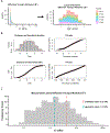
Figure 4:. Log-transformation of Young’s modulus data from mouse glial lamina.

A) Histogram of effective Young’s modulus values from 9 eyes of 5 mice. The raw data was log-transformed to obtain a distribution that appeared to be consistent with a normal distribution. Each color represents data from one animal. B) The log-transformed effective Young’s modulus values appeared to be well-fit by a normal distribution, as judged by a histogram of effective Young’s modulus values vs. a fitted normal distribution (top left), and by comparisons of actual and theoretical quantiles (top right), actual and theoretical cumulative distribution functions (bottom left), and actual and theoretical probability distributions (bottom right). In all four panels, actual data is in black/grey and theoretical fits are overlain in red. C) Histogram of effective Young’s modulus values showing geometric and arithmetic means. The geometric mean, indicated by the blue dashed line, better represents the data compared to the arithmetic mean. X-axis is shown on a log-scale.

References

1. Alcaraz J, Otero J, Jorba I, Navajas D, 2018. Bidirectional mechanobiology between cells and their local extracellular matrix probed by atomic force microscopy. Semin. Cell Dev. Biol., Application of Atomic Force Microscopy in cell biology 73, 71–81. 10.1016/j.semcdb.2017.07.020 - DOI - PubMed
1. Bae YH, Liu S, Byfield FJ, Janmey PA, Assoian RK, 2016. Measuring the Stiffness of Ex Vivo Mouse Aortas Using Atomic Force Microscopy. J. Vis. Exp. 54630. 10.3791/54630 - DOI - PMC - PubMed
1. Binnig G, Quate CF, Gerber Ch., 1986. Atomic Force Microscope. Phys. Rev. Lett. 56, 930–933. 10.1103/PhysRevLett.56.930 - DOI - PubMed
1. Boettcher HS, Knudsen JC, Andersen PH, Danscher AM, 2014. Technical note: Effects of frozen storage on the mechanical properties of the suspensory tissue in the bovine claw. J. Dairy Sci. 97, 2969–2973. 10.3168/jds.2013-7208 - DOI - PubMed
1. Bouchonville N, Meyer M, Gaude C, Gay E, Ratel D, Nicolas A, 2016. AFM mapping of the elastic properties of brain tissue reveals kPa μm−1 gradients of rigidity. Soft Matter 12, 6232–6239. 10.1039/C6SM00582A - DOI - PubMed
LinkOut - more resources