Frequency-dependent dynamics of steady-state visual evoked potentials under sustained flicker stimulation

Abstract

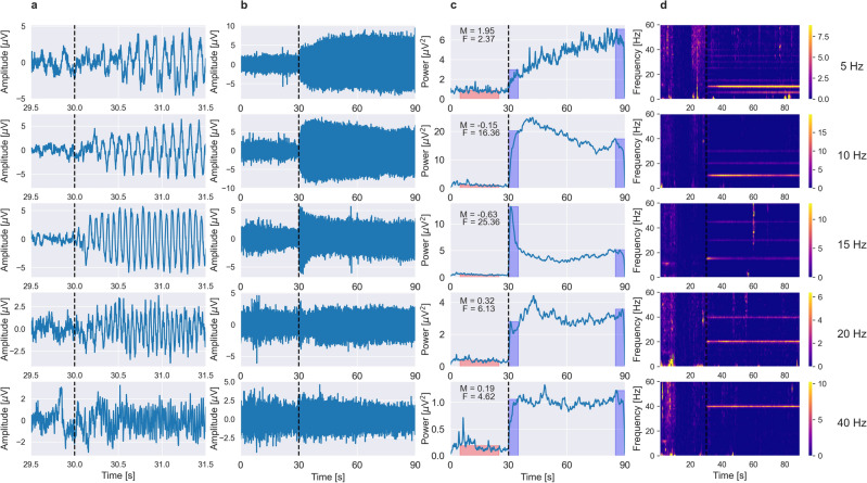
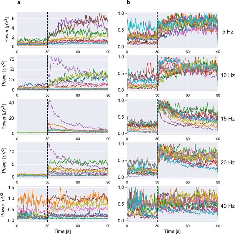
Steady-state visual evoked potentials (SSVEP) are electroencephalographic signals elicited when the brain is exposed to a visual stimulus with a steady frequency. We analyzed the temporal dynamics of SSVEP during sustained flicker stimulation at 5, 10, 15, 20 and 40 Hz. We found that the amplitudes of the responses were not stable over time. For a 5 Hz stimulus, the responses progressively increased, while, for higher flicker frequencies, the amplitude increased during the first few seconds and often showed a continuous decline afterward. We hypothesize that these two distinct sets of frequency-dependent SSVEP signal properties reflect the contribution of parvocellular and magnocellular visual pathways generating sustained and transient responses, respectively. These results may have important applications for SSVEP signals used in research and brain-computer interface technology and may contribute to a better understanding of the frequency-dependent temporal mechanisms involved in the processing of prolonged periodic visual stimuli.

Figure 1

The evolution of SSVEP signals for five visual stimulation frequencies in an exemplary subject. (a) The raw EEG around stimulus onset (dashed black vertical line), averaged across trials shows the transient onset response for the first 250–300 ms and build-up of rhythmic response afterward. (b) The raw EEG averaged across trials. On each plot, the first 30 s correspond to the rest period, and the next 60 s correspond to stimulation time. The dashed black vertical line indicates stimulation onset. (c) The instantaneous SSVEP power averaged over 50 trials. On each panel, values of facilitation, F and modulation, M indices (see section “Methods”) are provided in the upper left corner. Red and blue rectangles show evaluation periods (width) and estimated power values (height) in the baseline (P_baseline) and stimulation conditions (P_initial and P_final), respectively, used for F and M calculation. It can be seen that different stimulation frequencies lead to distinct temporal evolution patterns of the power of SSVEP signals. (d) The spectrograms showing relative power differences from baseline (10–20 s) in the SSVEP signals. The colorbar placed along the side of each subplot indicates the mapping of the relative spectral power values (in a.u.) to color. The fundamental and higher harmonic frequencies of SSVEP responses are apparent.

Figure 2

SSVEP power evolution in individual subjects. (a) Absolute power scale. (b) Normalized power scale. On each plot, the first 30 s correspond to the rest period, and the next 60 s correspond to stimulation time. The black vertical line indicates stimulation onset. Each panel corresponds to a stimulus frequency shown on the right. Each color represents SSVEP power changes in an individual subject. Despite differences in absolute SSVEP magnitude, the temporal trends in responses are specific for each frequency.

Figure 3

Values of the F index (i.e., the relative power increase during the first 5 s of stimulation) for different stimulation frequencies. Each red dot represents the F value of a single subject, at a given stimulus frequency. Each blue box extends from the first (q1) to the third (q3) quartile values of the data with a line at the median. The interquartile interval iqr = q3 − q1 contains 50% of the data. Whiskers of each boxplot indicate the highest and the lowest data value that is still within the lower q1 − 1.5 * iqr and upper q3 + 1.5 * iqr bound. Data found outside these boundaries are considered to be outliers and are shown as individual points. Significant differences were assessed by the Wilcoxon signed-rank test and are indicated by stars (*p < 0.05 and **p < 0.01).

Figure 4

The duration of fast (phasic) SSVEP facilitation quantified by the latency of the first maximum of the SSVEP signal power derivative. (a) The latency expressed in seconds, L_t. (b) The latency expressed as the number of cycles, L_c. Each red dot represents the latency value of a single subject, at a given stimulus frequency. In the boxplots, each blue box extends from the first (q1) to the third (q3) quartile values of the data with a line at the median. The interquartile interval iqr = q3 − q1 contains 50% of the data. Whiskers of each boxplot indicate the highest and the lowest data value that is still within the lower q1 − 1.5 * iqr and upper q3 + 1.5 * iqr bound. Data found outside these boundaries are considered to be outliers and are shown as individual points. Statistically significant differences were tested by the Wilcoxon signed-rank test and paired t-test and are indicated by stars (*p < 0.05).

Figure 5

The long-term power evolution of SSVEP quantified by the M index. Each red dot represents the modulation index M of a single subject, at a given stimulus frequency. In the boxplots, each blue box extends from the first (q1) to the third (q3) quartile values of the data with a line at the median. The interquartile range iqr = q3 − q1 contains 50% of the data. Whiskers of each boxplot indicate the highest and the lowest data value that is still within the lower q1 − 1.5 * iqr and upper q3 + 1.5 * iqr bound. Data found outside of these boundaries are considered to be outliers and are shown as individual points. Significant differences were assessed by the Wilcoxon signed-rank test and a paired t-test and are indicated by stars (*p < 0.05, **p < 0.01 and ***p < 0.001). The differences in M values across frequencies show that the long-term properties of SSVEP signals are frequency-dependent.

References

1. Berger H. Über das Elektrenkephalogramm des Menschen. Arch. Psychiatr. Nervenkr. 1929;87:527–570. doi: 10.1007/BF01797193. - DOI
1. Adrian ED, Matthews BHC. The Berger rhythm: Potential changes from the occipital lobes in man. Brain. 1934;57:355–385. doi: 10.1093/brain/57.4.355. - DOI - PubMed
1. Regan D. Some characteristics of average steady-state and transient responses evoked by modulated light. Electroencephalogr. Clin. Neurophysiol. 1966;20:238–248. doi: 10.1016/0013-4694(66)90088-5. - DOI - PubMed
1. Vialatte FB, Maurice M, Dauwels J, Cichocki A. Steady-state visually evoked potentials: Focus on essential paradigms and future perspectives. Prog. Neurobiol. 2010;90:418–438. doi: 10.1016/j.pneurobio.2009.11.005. - DOI - PubMed
1. Norcia AM, Gregory Appelbaum L, Ales JM, Cottereau BR, Rossion B. The steady-state visual evoked potential in vision research: A review. J. Vis. 2015;15:1–46. doi: 10.1167/15.6.4. - DOI - PMC - PubMed
Publication types