MCell4 with BioNetGen: A Monte Carlo simulator of rule-based reaction-diffusion systems with Python interface

Abstract

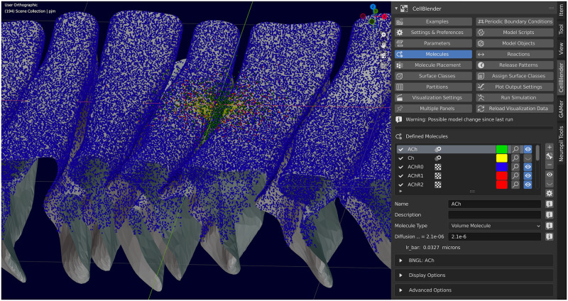
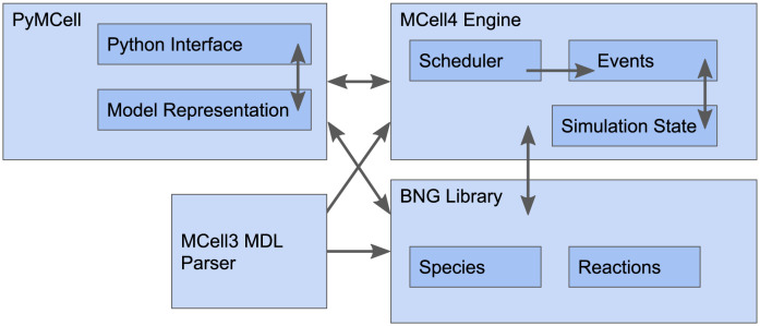
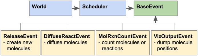
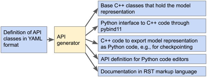
Biochemical signaling pathways in living cells are often highly organized into spatially segregated volumes, membranes, scaffolds, subcellular compartments, and organelles comprising small numbers of interacting molecules. At this level of granularity stochastic behavior dominates, well-mixed continuum approximations based on concentrations break down and a particle-based approach is more accurate and more efficient. We describe and validate a new version of the open-source MCell simulation program (MCell4), which supports generalized 3D Monte Carlo modeling of diffusion and chemical reaction of discrete molecules and macromolecular complexes in solution, on surfaces representing membranes, and combinations thereof. The main improvements in MCell4 compared to the previous versions, MCell3 and MCell3-R, include a Python interface and native BioNetGen reaction language (BNGL) support. MCell4's Python interface opens up completely new possibilities for interfacing with external simulators to allow creation of sophisticated event-driven multiscale/multiphysics simulations. The native BNGL support, implemented through a new open-source library libBNG (also introduced in this paper), provides the capability to run a given BNGL model spatially resolved in MCell4 and, with appropriate simplifying assumptions, also in the BioNetGen simulation environment, greatly accelerating and simplifying model validation and comparison.

Fig 1. Model creation with CellBlender.

MCell4 models can be created, executed, analyzed, and visualized using CellBlender, an addon for Blender. The capabilities of Blender are indispensable for creating complex geometries for MCell4 models.

Fig 2. Overview of MCell4 architecture.

MCell4 is comprised of four main components: 1) The PyMCell library provides a Python interface and contains classes to hold the model representation, 2) The MCell4 engine implements the simulation algorithms, 3) The BNG (BioNetGen) library provides methods to resolve BioNetGen reactions, and 4) The MDL (Model Description Language) parser enables backward compatibility with MCell3.

Fig 3. Overview of MCell4 Scheduler.

The Scheduler executes time step iterations which consist of discrete events executed in this order: 1) A ReleaseEvent creates new molecules, 2) A DiffuseReactEvent implements diffusion of molecules, checks collisions, and executes reactions, 3) A MolRxnCountEvent counts numbers of molecules or how many times a reaction occurs, and 4) A VizOutputEvent stores molecule locations for visualization in CellBlender. Only the DiffuseReactEvent must be executed at each time step to move the time forward. The other events listed here are optional.

Fig 4. Overview of MCell4 API generator.

When MCell4 is built from its source code, the API generator reads a high-level definition of the MCell4 Python interface and generates code and documentation. Automatic generation of an API makes it possible to easily modify or extend the API while ensuring that all parts including documentation stay consistent. While the generated C++ and pybind11 code are not directly relevant to users, the generated API definition for Python code editors (contained in the file mcell.pyi) enables code completion and parameter info features in Python editors that support it such as VSCode [25]. This is indispensable to users creating their own models using the MCell4 Python API. Furthermore, the generated end-user documentation provides necessary details on what classes and methods are offered [26]. Checkpointing stores the current state of simulation as an MCell4 model in Python that can be manually modified if needed. The API generator is a general tool that can also be used (with minor modifications) for other software tools that combine C++ and Python [27].

Fig 5. Recommended structure of a standard MCell4 model.

The main files included in a standard MCell4 model are: 1) parameters.py with all the model parameters, 2) subsystem.py that captures information on species and reactions in a way that is independent of a particular model and can be used as a reusable module, 3) geometry.py with a definition of 3D geometry objects, 4) instantiation.py that usually defines the initial model state, i.e., which geometry objects are created in the simulation and the number and positions of molecules to be released at a given time, 5) observables.py with lists of characteristics to be measured and saved in files during simulation, and 6) model.py in which all the parts of the model are assembled together and in which the the simulation loop with optional interactions with external simulators is defined. This recommended model structure is not enforced by MCell4 itself. However, use of this structure promotes readability, modularity, navigation, and sharing of models with others. The MCell4 Python code generator in CellBlender follows this recommended structure with the addition of a file called customization.py whose purpose is to provide a means to modify/expand the model in the case when the standard files are automatically generated from the CellBlender representation.

Fig 6. Example of model modularity.

Modularity of a model allows assembly of multiple subsystem definitions into a single model. In the example shown here, individual modules are assembled to construct a model of a new synaptic pathway that is affected by other processes. The complete model includes modules that individually define the presynaptic terminal with its presynaptic pathways and the postsynaptic spine with its postsynaptic pathways.

Fig 7. A simple MCell4 model.

Example of a simple MCell4 model that releases 10 volume molecules of species ‘a’ and simulates their diffusion for 10 iterations with a default time step of 1 μs. Note that for this and the following examples, a system variable, PYTHONPATH, must be set so that the Python interpreter knows where to find the MCell4 module. Further details are provided in the MCell4 Installation Documentation [29]. MCell4/CellBlender is provided as a bundle which includes Blender, CellBlender, and MCell4 all packaged together. Blender comes with its own Python built-in. MCell4 can use this Python.

Fig 8. Example of graph transformation with BNG reaction rules.

This example shows details of how BNG reactions are implemented in the libBNG library [19]. Reactants are defined with molecule types A(c0∼R∼S,c0∼R∼S) and B(c1∼U∼V,c2∼X∼Y) where A and B are names of the molecule types, c0 is a component of A that can be in one of the states R and S, and similarly c2 and c3 are components of B. (A) is the example reaction rule, (B) are example species reactants and products in the BNGL syntax, and (C) shows a graph representation of the rule in (B). Application of the rule is done in the following steps: 1) a mapping from each molecule and each component from reactant patterns (E) onto reactants (D) is computed (dotted arrows). If the state of a component is set in the pattern, the corresponding reactant’s component state must match. The next step 2) is to compute a mapping of the rule product pattern (F) onto reactant patterns (E). The difference between the reaction rule product pattern and the reactant patterns tells what changes need to be made to generate the product. In this example, a bond between A’s component c0 with state R and B’s component c1 is created. The state of A’s component c0 is changed to S. Once the mappings are computed, we follow the arrows leading from the reaction rule product pattern (F) to reactant patterns (E) and then to reactants (D) and 3) perform changes on the reactants resulting in the product graph (G). Each graph component of the product graph is a separate product and there is exactly one product in this example.

Fig 9. Example of compartments.

EC is extracellular space, PM is the plasma membrane, and CP is cytoplasm. A is a molecule that diffuses freely in 3D space, and T is a molecule located in the plasma membrane.

Fig 10. Example model using BNGL.

BNGL file that defines a compartment CP, and instantiates release of 100 molecules of A and 100 molecules of B into it. It then implements a reaction rule in which A and B react to form the product C.

Fig 11. Example of loading and running BNGL model in MCell4.

Python code for an MCell4 model that will implement loading of the BNGL file shown in Fig 10 (referenced as subsystem.bngl). In this example the entire BNGL file is read. It is also possible to load only specific parts of the BNGL file, for example only reaction rules or only compartment and molecule release information. It is also possible to replace BNGL compartments with actual 3D geometry.

Fig 12. Compartmental BNGL implementation of the SNARE complex model.

One 3D compartment, cytosol (CP), and its associated plasma membrane (PM) are defined. Molecule types are defined, and their released sites are specified: SNARE molecules are released into the PM, and Calcium ions into the Cytosol. This code is followed by specification of the observables, and the reaction rules governing the interactions.

Fig 13. Validation of model of the SNARE complex.

(A) Schematic diagram of the state variables of the SNARE complex model. It consists of a total of 36 states: 18 with a docked vesicle and 18 without a docked vesicle. The 2 separate vesicle states are not shown in the diagram. S and A represent the synchronous and asynchronous components of the complex, which can be in 6 and 3 different states respectively. (B-D) Results of independent simulations of the model with ODEs in BioNetGen (dashed lines) and in MCell4 (solid lines).

Fig 14. Validation of MCell4 simulation against BioNetGen/NFsim and MCell3R using a model of CaMKII.

The input BNGL model for NFsim was obtained by automatic BNGL export of BNGL from the MCell4 model. The simulation ran for 100000 iterations (0.1 s). Lines in the graphs are averages from 256 runs with different random seeds, and bands represent one standard deviation. Molecules in MCell3R and MCell4 use diffusion constant of 10⁻³cm²/s to emulate a well-mixed solution (the usual value is around 10⁻⁶cm²/s). The names of the observed species are indicated in the graph titles: A) Ca is unbound calcium ions; B) CaM1C is CaM(C∼1, N∼0, camkii); C) CaM1N is CaM(C∼0, N∼1, camkii); D) KCaM2N is CaMKII(T286∼U, cam!1).CaM(C∼0, N∼2, camkii!1). The simulation was initiated far from equilibrium; therefore there was an initial jump in the molecule numbers. The molecule names are explained in [40].

Fig 15. The effect on CaMKII phosphorylation of trapping CaMKII and CaM inside the PSD of a dendritic spine head.

Three different conditions were simulated within a compartment representing a dendritic spine head containing a subcompartment representing a postsynaptic density (PSD) shown in panel D. (A) All molecules are homogeneously distributed throughout the entire spine head. The PSD is made to be transparent to the diffusion of all molecules. (B) The PSD is made to be reflective to CaMKII and CaM, but transparent to calcium ions and PP1. All the molecules are homogeneously distributed throughout both compartments. (C) The PSD is made to be reflective to CaMKII and CaM and 50% of the CaMKII molecules are trapped inside the PSD, while the rest of the molecules are distributed homogeneously throughout the remainder of the spine head. D) Diagram of the spine head compartment 0.5 x 0.5 x 0.5 um in size containing the PSD subcompartment 0.05 x 0.4 x 0.4 um in size. The plots show an average of 60 runs, lighter-shaded bands represent the standard error of the mean.

Fig 16. Simulation of membrane localization.

The plot shows copy numbers of a surface molecule MA (surface molecule M with a bound volume molecule A). MCell4 and MCell3 results show a good match with simulations using the NERDSS simulator (NERDSS results are from from [41]) and with simulations in VCell using a PDE method (VCell results are from from [41]). Results of simulations with an ODE method in VCell differ from MCell3, MCell4, NERDSS, and PDE solutions. MCell3 and MCell4 results are an average of 512 runs with different random seeds.

Fig 17. Simulation of a system that exhibits stochastic switching between multiple steady states.

Copy numbers of unphosphorylated kinase A and its phosphorylated variant Ap are shown for a single simulation run in: A) MCell4; B) MCell3; and C) NFsim. The NFsim model was obtained by automatically exporting the MCell4 model into BNGL. The graphs also show solutions obtained with a deterministic ODE model for which data from [41] were used. The results demonstrate that the MCell results correctly reach one of the stable steady states shown in the ODE results. The simulation stays in such a state, and then due to stochastic behavior, a switch another steady state occurs.

Fig 18. Performance benchmarks of MCell4.

For selected benchmarks, we measured elapsed time for how long the simulation ran starting from the second iteration (after all initializations) and ending when the simulation finished. Time was measured on AMD Ryzen 9 3900X@3.8GHz. Both MCell3 and MCell4 use a single execution thread. Relative performance shown in the graphs is computed as time for MCell3 (panel A) or MCell3-R (panel B) divided by time for MCell4. The sources of the models are as follows: Presynaptic Ca Homeostasis [39]; Rat Neuromuscular Junction [2] model with updated geometry (shown in Fig 1), Neuropil [5]; Mitochondrion Model [47]; Membrane Localization [41]; Autophosphorylation [41]; CaMKII Monomers [40]; CaMKII Holoenzyme [40]; SynGAP and TARP with the PDZ domains of PSD-95 (MCell4 model not yet published).

Fig 19. Reaction rules affecting repressor protein R in the particle-only model.

Fig 20. Reaction rules affecting repressor protein R in the hybrid model.

Fig 21. Pseudo-code of the main simulation loop.

This script in pseudo-code: 1) runs an iteration of the particle-based simulation, 2) updates the copy number of R based on the current MCell4 state, and 3) updates the rate of reaction A -> AR that was originally a bimolecular reaction A + R -> AR. N is a unit representing the copy number. This pseudo-code was adapted to show the actual computations in a more comprehensible way. The runnable MCell4 Python code is available in the GitHub repository accompanying this article [37].

Fig 22. Simulation of a circiadian clock.

(A) Result of a stochastic simulation of a circadian clock model with NFsim. Copy numbers of molecules A and R show periodic oscillation. A low pass frequency filter was used to smooth the values of A and R. The reason for the smoothing was to get a numerical value related to the actual peak. The peaks from low-pass filtered data do not represent true average peaks but can be used as a proxy to obtain the time of a peak for comparison with other simulation methods. (B) The error bars capture the mean and standard deviation of the low pass filtered peak times for different variants of the model and simulation algorithms. Each of the variants was run 1024 times. It is evident that the SSA, the NFsim, and the MCell4 model variants with a fast diffusion constant, D = 10⁻⁵ cm²/s, give essentially the same results. The hybrid MCell4 model with the slower diffusion constant, D = 10⁻⁷ cm²/s, shows faster oscillation than the non-spatial models run with SSA and NFsim, and the MCell4 variants with faster diffusion. The pure particle-based MCell4 model with D = 10⁻⁷cm²/s shows the fastest oscillations.

Fig 23. Comparison of copy numbers of A and R during simulations by different methods.

(A) The average copy numbers for A and R proteins from 1024 runs in NFsim, SSA, and MCell4 with a fast diffusion constant match. To get an even better match, would require more than 1024 runs because stochastic molecular simulations show high variability when the copy number of some of the species is low which is the case here for both A and R. (B) and (C) Average copy numbers for MCell4 simulations with a slow diffusion constant. These are shown as separate plots to highlight the effect of slow diffusion on spatial simulation results.

References

1. Gunawardena J. Models in biology:‘accurate descriptions of our pathetic thinking’. BMC biology. 2014;12(1):1–11. doi: 10.1186/1741-7007-12-29 - DOI - PMC - PubMed
1. Stiles JR, Van Helden D, Bartol TM, Salpeter MM. Miniature endplate current rise times < 100 μs from improved dual recordings can be modeled with passive acetylcholine diffusion from a synaptic vesicle. Proc Natl Acad Sci. 1996;93(12):5747–5752. doi: 10.1073/pnas.93.12.5747 - DOI - PMC - PubMed
1. Stiles JR, Bartol TM. 4. In: Schutter E, editor. Monte Carlo Methods for Simulating Realistic Synaptic Microphysiology Using MCell. CRC Press; 2001.
1. Kerr RA, Bartol TM, Kaminsky B, Dittrich M, Chang JCJ, Baden SB, et al.. Fast Monte Carlo simulation methods for biological reaction-diffusion systems in solution and on surfaces. SIAM journal on scientific computing. 2008;30(6):3126–3149. doi: 10.1137/070692017 - DOI - PMC - PubMed
1. Bartol TM, Keller DX, Kinney JP, Bajaj CL, Harris KM, Sejnowski TJ, et al.. Computational reconstitution of spine calcium transients from individual proteins. Frontiers in synaptic neuroscience. 2015;7:17. doi: 10.3389/fnsyn.2015.00017 - DOI - PMC - PubMed
Publication types