Thermodynamic analog of integrate-and-fire neuronal networks by maximum entropy modelling

Abstract

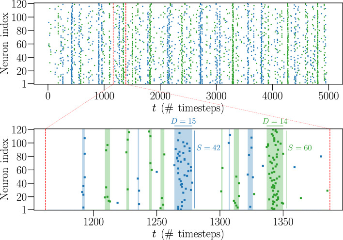
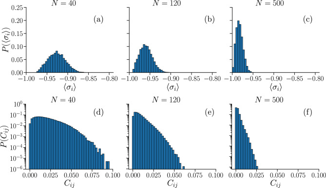
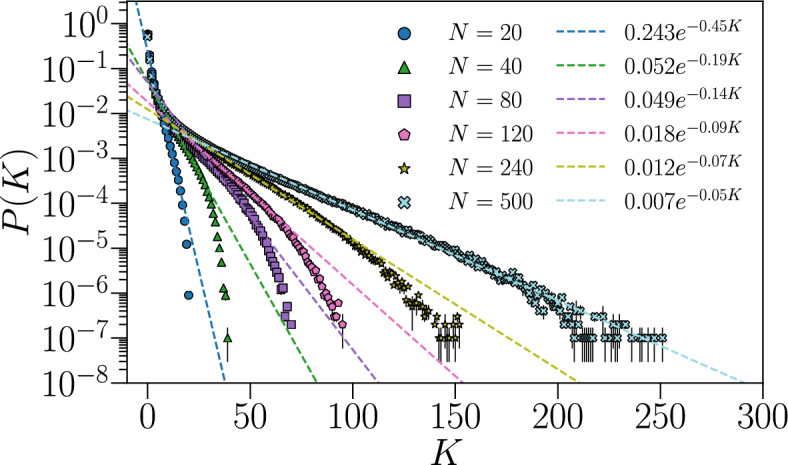
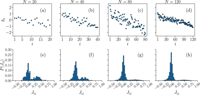
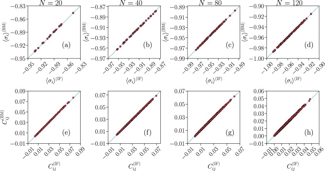
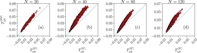
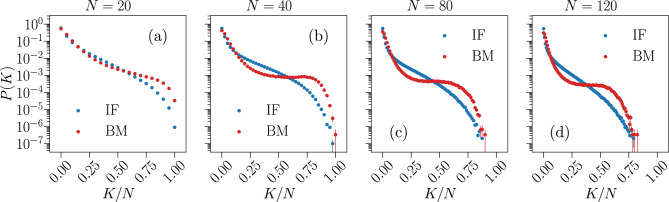
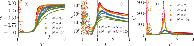
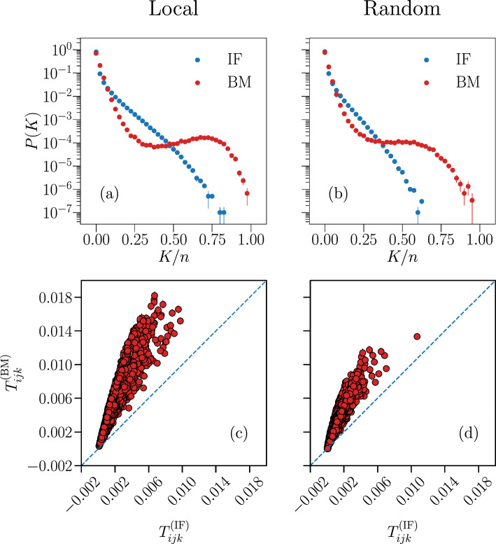
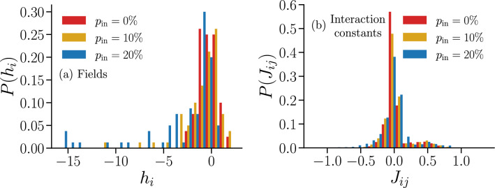
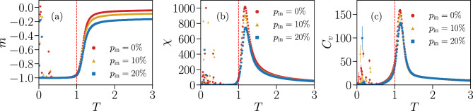
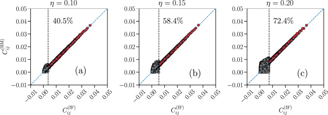
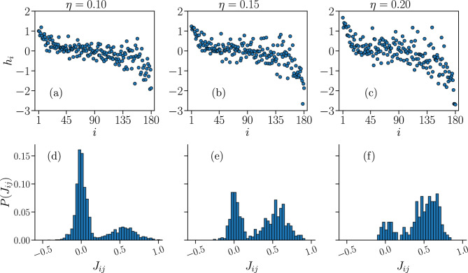
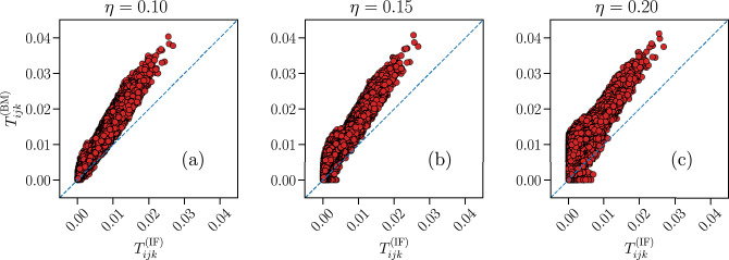
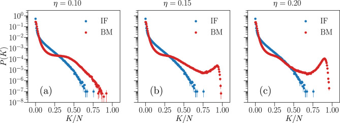
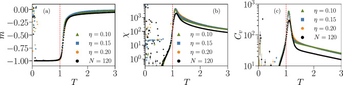
Recent results have evidenced that spontaneous brain activity signals are organized in bursts with scale free features and long-range spatio-temporal correlations. These observations have stimulated a theoretical interpretation of results inspired in critical phenomena. In particular, relying on maximum entropy arguments, certain aspects of time-averaged experimental neuronal data have been recently described using Ising-like models, allowing the study of neuronal networks under an analogous thermodynamical framework. This method has been so far applied to a variety of experimental datasets, but never to a biologically inspired neuronal network with short and long-term plasticity. Here, we apply for the first time the Maximum Entropy method to an Integrate-and-fire (IF) model that can be tuned at criticality, offering a controlled setting for a systematic study of criticality and finite-size effects in spontaneous neuronal activity, as opposed to experiments. We consider generalized Ising Hamiltonians whose local magnetic fields and interaction parameters are assigned according to the average activity of single neurons and correlation functions between neurons of the IF networks in the critical state. We show that these Hamiltonians exhibit a spin glass phase for low temperatures, having mostly negative intrinsic fields and a bimodal distribution of interaction constants that tends to become unimodal for larger networks. Results evidence that the magnetization and the response functions exhibit the expected singular behavior near the critical point. Furthermore, we also found that networks with higher percentage of inhibitory neurons lead to Ising-like systems with reduced thermal fluctuations. Finally, considering only neuronal pairs associated with the largest correlation functions allows the study of larger system sizes.

Figure 1

Time series for a system at criticality with $N=120$ neurons. The top raster plot presents the time evolution of the firing states of $N=120$ neurons over a certain number of timesteps, from a fully-excitatory IF network in the critical state. A coloured dot indicates that the respective neuron fired during that timestep, while an absence of a dot means it was inactive. The alternating green and blue colours are just a visual aid to distinguish between different avalanches. The bottom raster plot is a zoom-in of the top one, where the coloured shaded areas indicate avalanches of size $S>1$ and duration D.

Figure 2

Distributions of the average local activity $⟨{\sigma }_i⟩$ and of the correlation functions $C_{\mathit{ij}}$ in IF networks. Average local activity $⟨{\sigma }_i⟩$ (a–c) and correlation functions $C_{\mathit{ij}}$ (d–f), calculated as averages over $N_b={10}^7$ time bins. Distributions are obtained for sizes $N=\{40,120,500\}$, for $N_c\sim 10,000/N$ different fully-excitatory networks.

Figure 3

Probability P(K) of observing K neurons firing simultaneously during a time bin $\mathrm{\Delta }{t}_b=5$ timesteps. Results are averaged over $N_c$ different fully-excitatory IF networks configurations of size N. $N_c$ varies with N as in Fig. 2. For each configuration, P(K) is estimated by averaging over $N_b={10}^7$ bins. Error bars are given by the standard error, and most of them are smaller than the symbol size.

Figure 4

Sets of learned fields $h_i$ and interaction constants $J_{\mathit{ij}}$ of the Ising model reproducing the time averages of the IF model. Plots of the fields $h_i$ (a–d), sorted by the average local activity ${⟨{\sigma }_i⟩}^{\text{(IF)}}$ of the associated neuron i, in order of decreasing ${⟨{\sigma }_i⟩}^{\text{(IF)}}$, and distributions of the interaction constants $J_{\mathit{ij}}$ (e–h), learned by the BM to reproduce the average local activity $⟨{\sigma }_i⟩$ and two-point correlation functions $C_{\mathit{ij}}$ of a fully-excitatory IF neural network at criticality, with $N=\{20,40,80,120\}$ neurons.

Figure 5

Quality test for the BM learning process. Comparison between the average local activity $⟨{\sigma }_i⟩$ (a–d) and correlation functions $C_{\mathit{ij}}$ (e–h) of the Ising-like model (y-axes) and IF model network (x-axes), for system sizes $N=\{20,40,80,120\}$. The blue dashed lines are the bisector $y=x$. Results are averages over $N_b={10}^7$ time bins for the IF model (IF), and over $M_c=3·{10}^6$ spin configurations for the Ising model (BM). Error bars are given by the standard error, and are smaller or equal to the symbol size.

Figure 6

Predictive capability of the Ising model for the three-point correlation functions $T_{\mathit{ijk}}$. Comparison between the three-point correlation functions $T_{\mathit{ijk}}$ of the Ising-like model (y-axes) and the IF model network (x-axes), for system sizes $N=\{20,40,80,120\}$. The blue dashed lines are the bisector $y=x$. Results are averages over $N_b={10}^7$ time bins for the IF model (IF), and over $M_c=3·{10}^6$ spin configurations for the Ising model (BM). Error bars are given by the standard error, and are smaller or equal to the symbol size.

Figure 7

Predictive capability of the Ising model for the probability of simultaneous firing P(K). Comparison between the simultaneous firing/up-state probability P(K) of the Ising-like model (red) and the IF model network (blue), for system sizes $N=\{20,40,80,120\}$. Results are averaged over $N_b={10}^7$ time bins for the IF model (IF), and over $M_c=3·{10}^6$ spin configurations for the Ising model (BM). Error bars are given by the standard error, and most are smaller or equal to the symbol size.

Figure 8

Thermodynamic functions of Ising models associated with fully-excitatory IF networks of different system sizes N. Average magnetization per spin m (a), susceptibility $\chi$ (b) and specific heat $C_v$ (c) as a function of the temperature $T\in [0.1,3.0]$, for systems with $N=\{20,40,80,120\}$ spins. Different curves with the same colour and symbol correspond to Ising systems with parameters fitted to different IF network configurations with the same size N but different specific connectivities. The vertical dashed lines indicate $T=T_0=1$, the “default” temperature used in the BM learning procedure to fit the respective Ising parameters to each IF network. The cloud of random values observed for $T<1$ suggests the presence of a spin-glass phase, where the thermal energy is insufficient to drive the system away from the initial random spin configuration. Results are averages over $M_c=3·{10}^6$ spin configurations. Error bars are given by the standard error and are overall smaller or equal to the symbol size.

Figure 9

Schematic representations of IF model subnetworks with different spatial distribution. Subnetworks (green) with neurons closely packed together (a) or picked at random positions (b). Subnetworks have $n=40$ neurons in a system of size $N=500$.

Figure 10

Predictive capability of the Ising model for IF model subnetworks. Comparison between Monte Carlo sampling of the Ising model (BM) and the neural network data (IF) of the probability P(K) (a,b) and triplets $T_{\mathit{ijk}}$ (c,d), for subnetworks with $n=40$ neurons, with a local (a,c) and random (b,d) spatial distribution, in a system with $N=500$ neurons. The blue dashed lines in the bottom plots are the bisector $y=x$. Results are averaged over $N_b={10}^7$ time bins for the IF model (IF), and over $M_c=3·{10}^6$ spin configurations for the Ising model (BM). Error bars are given by the standard error, and are overall smaller or equal to the symbol size.

Figure 11

Distributions of the learned fields $h_i$ and interaction constants $J_{\mathit{ij}}$ of a Ising model for neural networks with different fractions of inhibitory neurons $p_{\text{in}}$. Fields $h_i$ (a) and interaction constants $J_{\mathit{ij}}$ (b) associated with IF networks with $p_{\text{in}}=\{0\%,10\%,20\%\}$ and $N=80$, obtained after $N_{\text{BM}}=60,000$ iterations of the BM.

Figure 12

Thermodynamic functions of Ising-like models associated with IF model networks with different fractions of inhibitory neurons $p_{\text{in}}$. Average magnetization per spin m (a), susceptibility $\chi$ (b) and specific heat $C_v$ (c) as a function of the temperature $T\in [0.1,3.0]$, simulated using the learned parameters shown in Fig. 11 for different fractions of inhibitory neurons $p_{\text{in}}=\{0\%,10\%,20\%\}$ and $N=80$. As in Fig. 8, the cloud of random values for $T<1$ suggests the presence of a spin-glass phase. Results are averaged over $M_c=3·{10}^6$ spin configurations. Error bars are given by the standard error and are overall smaller or equal to the symbol size.

Figure 13

Quality test for the BM learning process with a partially-connected Ising model. Comparison between the correlation functions $C_{\mathit{ij}}$ of the partially-connected Ising-like model (y-axes) and IF model network (x-axes), for a fully-excitatory system at criticality of size $N=180$ and three different thresholds $\eta =\{0.10,0.15,0.20\}$ for the removal of the $J_{\mathit{ij}}$. If $C_{\mathit{ij}}^{\text{(IF)}}<\eta \text{max}(C_{\mathit{ij}}^{\text{(IF)}})$ (grey dots), the corresponding interaction constant is set to $J_{\mathit{ij}}=0$. The vertical dashed lines indicate the value $\eta \text{max}(C_{\mathit{ij}}^{\text{(IF)}})$, with the corresponding approximate percentage of removed $J_{\mathit{ij}}$ reported at the right of this line. The blue dashed lines are the bisector $y=x$. Results are averaged over $N_b={10}^7$ time bins for the IF model (IF), and over $M_c=3·{10}^7$ spin configurations for the Ising model (BM). Error bars are given by the standard error, and are smaller or equal to the symbol size.

Figure 14

Sets of learned fields $h_i$ and non-zero interaction constants $J_{\mathit{ij}}$ of the partially-connected Ising model. Plots of the fields $h_i$ (a–c), sorted by the average local activity ${⟨{\sigma }_i⟩}^{\text{(IF)}}$ of the associated neuron i, in order of decreasing ${⟨{\sigma }_i⟩}^{\text{(IF)}}$, and distributions of the non-zero interaction constants $J_{\mathit{ij}}$ (d–f), that reproduce the respective data of the Ising model presented in Fig. 13 for the three different thresholds $\eta =\{0.10,0.15,0.20\}$, for a fully-excitatory system at criticality of size $N=180$.

Figure 15

Predictive capability of the partially-connected Ising model for the three-point correlation functions $T_{\mathit{ijk}}$. Comparison between the three-point correlation functions $T_{\mathit{ijk}}$ of the partially-connected Ising-like model (y-axes) and the IF network (x-axes), for the three thresholds $\eta =\{0.10,0.15,0.20\}$, for a fully-excitatory system at criticality of size $N=180$. Results are averaged over $N_b={10}^7$ time bins for the IF model (IF), and over $M_c=3·{10}^7$ spin configurations for the Ising model (BM). Error bars are given by the standard error, and most are smaller or equal to the symbol size.

Figure 16

Predictive capability of the partially-connected Ising model for the probability of simultaneous firing P(K). Comparison between the simultaneous firing/up-state probability P(K) of the Ising-like model (red) and the IF model network (blue), for the three thresholds $\eta =\{0.10,0.15,0.20\}$, for a fully-excitatory system at criticality of size $N=180$. Results are averaged over $N_b={10}^7$ time bins for the IF model (IF), and over $M_c=3·{10}^7$ spin configurations for the Ising model (BM). Error bars are given by the standard error, and most are smaller or equal to the symbol size.

Figure 17

Thermodynamic functions of partially-connected Ising models associated with an IF model network with $N=180$. Average magnetization per spin m (a), susceptibility $\chi$ (b) and specific heat $C_v$ (c) as a function of the temperature $T\in [0.1,3.0]$, simulated using the learned parameters shown in Fig. 14 for the three different thresholds $\eta =\{0.10,0.15,0.20\}$, for a fully-excitatory IF network at criticality of size $N=180$. The black symbols show the results for a learned Ising model associated with an IF network of size $N=120$, considering the full set $\{J_{\mathit{ij}}\}$. As in Figs. 8 and 12, the cloud of random values for $T<1$ suggests the presence of a spin-glass phase. Results are averaged over $M_c=3·{10}^6$ spin configurations. Error bars are given by the standard error and are overall smaller or equal to the symbol size.

References

1. Hodgkin AL, Huxley AF. A quantitative description of membrane current and its application to conduction and excitation in nerve. J. Physiol. 1952;117:500. doi: 10.1113/jphysiol.1952.sp004764. - DOI - PMC - PubMed
1. Dayan, P. & Abbott, L. F. Theoretical Neuroscience: Computational and Mathematical Modeling of Neural Systems (The MIT Press, 2005).
1. Little WA. The existence of persistent states in the brain. Math. Biosci. 1974;19:101–120. doi: 10.1016/0025-5564(74)90031-5. - DOI
1. Hopfield JJ. Neural networks and physical systems with emergent collective computational abilities. Proc. Natl. Acad. Sci. 1982;79:2554–2558. doi: 10.1073/pnas.79.8.2554. - DOI - PMC - PubMed
1. Amit DJ, Gutfreund H, Sompolinsky H. Spin-glass models of neural networks. Phys. Rev. A. 1985;32:1007–1018. doi: 10.1103/PhysRevA.32.1007. - DOI - PubMed