Representing Context and Priority in Working Memory

Abstract

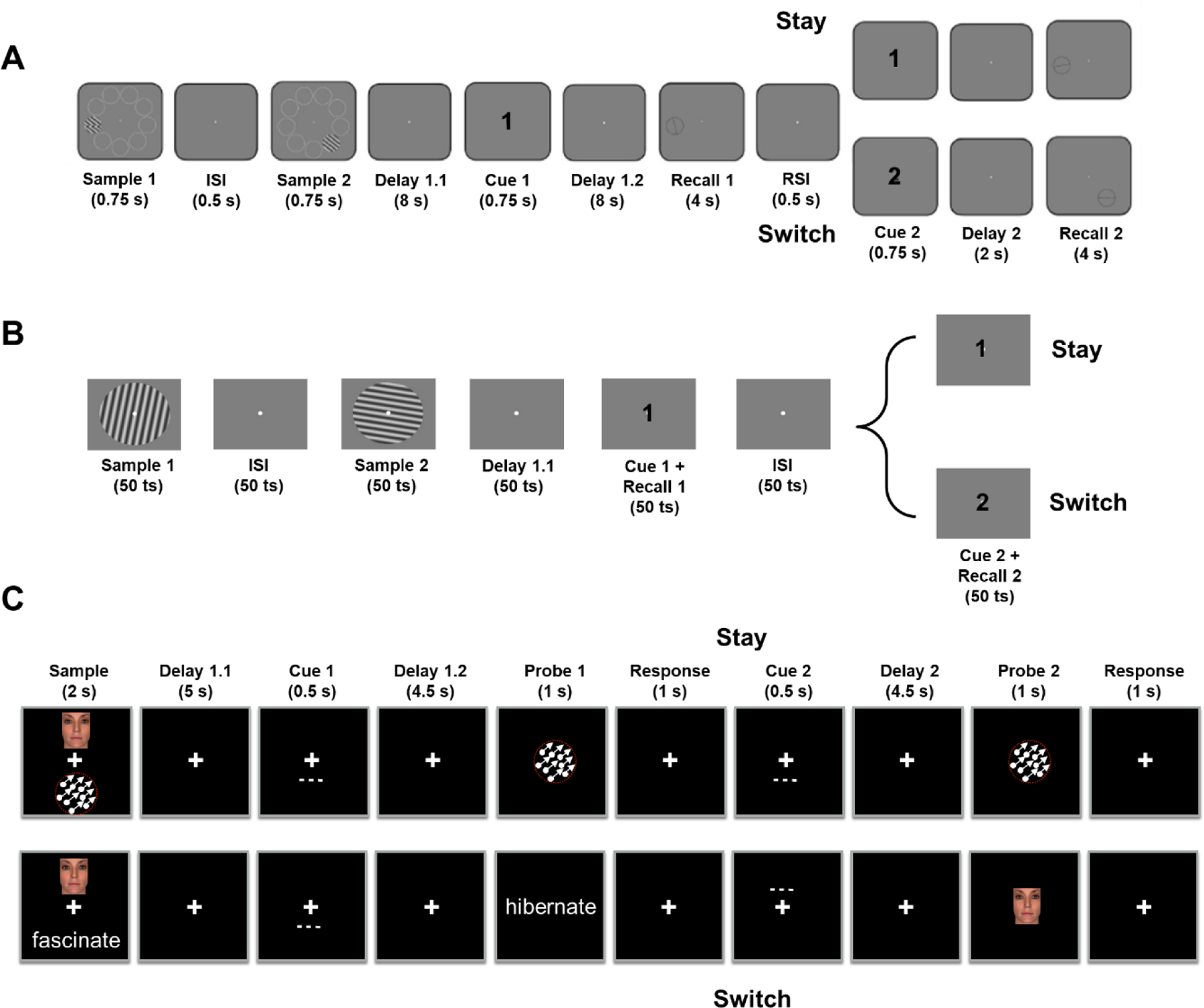
The ability to prioritize among contents in working memory (WM) is critical for successful control of thought and behavior. Recent work has demonstrated that prioritization in WM can be implemented by representing different states of priority in different representational formats. Here, we explored the mechanisms underlying WM prioritization by simulating the double serial retrocuing task with recurrent neural networks. Visualization of stimulus representational dynamics using principal component analysis revealed that the network represented trial context (order of presentation) and priority via different mechanisms. Ordinal context, a stable property lasting the duration of the trial, was accomplished by segregating representations into orthogonal subspaces. Priority, which changed multiple times during a trial, was accomplished by separating representations into different strata within each subspace. We assessed the generality of these mechanisms by applying dimensionality reduction and multiclass decoding to fMRI and EEG data sets and found that priority and context are represented differently along the dorsal visual stream and that behavioral performance is sensitive to trial-by-trial variability of priority coding, but not context coding.

Figure 1.

Experimental procedure for (A) The fMRI task, (B) the RNN task and (C) the EEG task. Figures adapted, with permission, from Yu, Teng, & Postle (2020; panel A), Fulvio and Postle (2020; panel C).

Figure 2.

RNN input and architecture. Top left illustrates input of a stimulus (either Sample 1 or Sample 2) with an angular value corresponding to the peak magnitude of this 32-dimensional vector; bottom left illustrates that at each timestep the value of the input to the cue input unit was 0, 1, or -1.

Figure 3.

Visualization of representational dynamics embedded in hidden layer of RNN #3 at each of five representative timesteps across the DSR task. Each plot contains 1000 data points, one corresponding to each simulated trial, and the symbols indicating that trial’s cue configuration: Cue 1 -> Sample 1, Cue 2 -> Sample 1(●); Cue 1 -> Sample 1, Cue 2 -> Sample 2 (▲); Cue 1 -> Sample 2, Cue 2 -> Sample 1 (■); Cue 1 -> Sample 2, Cue 2 -> Sample 2 (+). In each plot, an example trial of each cue configuration is colored black for better visualization. For each of the five timesteps the same data are illustrated in six ways: the top row with the data labeled as Sample 1 and the bottom row with the data labeled as Sample 2, and for each they are projected into three subspaces. A. After the presentation of Sample 1 (Timestep 99). Note that because Sample 2 has not yet been presented, the stimulus values are haphazard. B. After the presentation of Sample 2 (Timestep 199). With both items in WM, but prior to cuing, Sample 1 is now represented in the PC3-PC4 subspace and Sample 2 in the PC1-PC2 subspace. C. During presentation of Cue 1 and generation of Recall 1 (Timestep 214), illustrating a separation-by-priority status in the PC1-PC2 subspace. (A comparable priority-based separation was visible in the PC3-PC4 subspace earlier during this same epoch (not shown).) D. During the delay between Cue 1 and Cue 2 (Timestep 298). E. During presentation of Cue 2 and generation of Recall 2 (Timestep 312), again illustrating a separation-by-priority status in the PC1-PC2 subspace but now based on Cue 2. (As with the Cue 1 epoch, a comparable priority-based separation was visible in the PC3-PC4 subspace earlier during this Cue 2 epoch (not shown).)

Figure 3.

Visualization of representational dynamics embedded in hidden layer of RNN #3 at each of five representative timesteps across the DSR task. Each plot contains 1000 data points, one corresponding to each simulated trial, and the symbols indicating that trial’s cue configuration: Cue 1 -> Sample 1, Cue 2 -> Sample 1(●); Cue 1 -> Sample 1, Cue 2 -> Sample 2 (▲); Cue 1 -> Sample 2, Cue 2 -> Sample 1 (■); Cue 1 -> Sample 2, Cue 2 -> Sample 2 (+). In each plot, an example trial of each cue configuration is colored black for better visualization. For each of the five timesteps the same data are illustrated in six ways: the top row with the data labeled as Sample 1 and the bottom row with the data labeled as Sample 2, and for each they are projected into three subspaces. A. After the presentation of Sample 1 (Timestep 99). Note that because Sample 2 has not yet been presented, the stimulus values are haphazard. B. After the presentation of Sample 2 (Timestep 199). With both items in WM, but prior to cuing, Sample 1 is now represented in the PC3-PC4 subspace and Sample 2 in the PC1-PC2 subspace. C. During presentation of Cue 1 and generation of Recall 1 (Timestep 214), illustrating a separation-by-priority status in the PC1-PC2 subspace. (A comparable priority-based separation was visible in the PC3-PC4 subspace earlier during this same epoch (not shown).) D. During the delay between Cue 1 and Cue 2 (Timestep 298). E. During presentation of Cue 2 and generation of Recall 2 (Timestep 312), again illustrating a separation-by-priority status in the PC1-PC2 subspace but now based on Cue 2. (As with the Cue 1 epoch, a comparable priority-based separation was visible in the PC3-PC4 subspace earlier during this Cue 2 epoch (not shown).)

Figure 3.

Visualization of representational dynamics embedded in hidden layer of RNN #3 at each of five representative timesteps across the DSR task. Each plot contains 1000 data points, one corresponding to each simulated trial, and the symbols indicating that trial’s cue configuration: Cue 1 -> Sample 1, Cue 2 -> Sample 1(●); Cue 1 -> Sample 1, Cue 2 -> Sample 2 (▲); Cue 1 -> Sample 2, Cue 2 -> Sample 1 (■); Cue 1 -> Sample 2, Cue 2 -> Sample 2 (+). In each plot, an example trial of each cue configuration is colored black for better visualization. For each of the five timesteps the same data are illustrated in six ways: the top row with the data labeled as Sample 1 and the bottom row with the data labeled as Sample 2, and for each they are projected into three subspaces. A. After the presentation of Sample 1 (Timestep 99). Note that because Sample 2 has not yet been presented, the stimulus values are haphazard. B. After the presentation of Sample 2 (Timestep 199). With both items in WM, but prior to cuing, Sample 1 is now represented in the PC3-PC4 subspace and Sample 2 in the PC1-PC2 subspace. C. During presentation of Cue 1 and generation of Recall 1 (Timestep 214), illustrating a separation-by-priority status in the PC1-PC2 subspace. (A comparable priority-based separation was visible in the PC3-PC4 subspace earlier during this same epoch (not shown).) D. During the delay between Cue 1 and Cue 2 (Timestep 298). E. During presentation of Cue 2 and generation of Recall 2 (Timestep 312), again illustrating a separation-by-priority status in the PC1-PC2 subspace but now based on Cue 2. (As with the Cue 1 epoch, a comparable priority-based separation was visible in the PC3-PC4 subspace earlier during this Cue 2 epoch (not shown).)

Figure 3.

Visualization of representational dynamics embedded in hidden layer of RNN #3 at each of five representative timesteps across the DSR task. Each plot contains 1000 data points, one corresponding to each simulated trial, and the symbols indicating that trial’s cue configuration: Cue 1 -> Sample 1, Cue 2 -> Sample 1(●); Cue 1 -> Sample 1, Cue 2 -> Sample 2 (▲); Cue 1 -> Sample 2, Cue 2 -> Sample 1 (■); Cue 1 -> Sample 2, Cue 2 -> Sample 2 (+). In each plot, an example trial of each cue configuration is colored black for better visualization. For each of the five timesteps the same data are illustrated in six ways: the top row with the data labeled as Sample 1 and the bottom row with the data labeled as Sample 2, and for each they are projected into three subspaces. A. After the presentation of Sample 1 (Timestep 99). Note that because Sample 2 has not yet been presented, the stimulus values are haphazard. B. After the presentation of Sample 2 (Timestep 199). With both items in WM, but prior to cuing, Sample 1 is now represented in the PC3-PC4 subspace and Sample 2 in the PC1-PC2 subspace. C. During presentation of Cue 1 and generation of Recall 1 (Timestep 214), illustrating a separation-by-priority status in the PC1-PC2 subspace. (A comparable priority-based separation was visible in the PC3-PC4 subspace earlier during this same epoch (not shown).) D. During the delay between Cue 1 and Cue 2 (Timestep 298). E. During presentation of Cue 2 and generation of Recall 2 (Timestep 312), again illustrating a separation-by-priority status in the PC1-PC2 subspace but now based on Cue 2. (As with the Cue 1 epoch, a comparable priority-based separation was visible in the PC3-PC4 subspace earlier during this Cue 2 epoch (not shown).)

Figure 4.

The time course of effective dimensionality (ED) of the hidden layer stimulus representations of RNN #3. The rectangular images above the curve denote corresponding task events. The black rectangles along the x-axis indicate time periods when a response was being made. (See Appendix Figure A3 for effective dimensionality time courses from other networks.)

Figure 5.

Transformational variability analysis results on fMRI (Yu, Teng, & Postle, 2020) and EEG (Fulvio & Postle, 2020) data. (A) Comparisons between average TVI for high-error and low-error trials across subjects from the fMRI dataset. (B) Comparisons between average TVI for incorrect and correct trials across subjects from the EEG dataset. Top row: priority-based decoding; bottom row: context-based decoding. The subspace from which the TVI is calculated is indicated in the legends. Asterisks above bars of the same color indicate the significance level of the paired-sample t tests comparing the average TVI between each two groups.

Figure 6.

Within- and cross-label decoding of stimulus identity averaged across the ten RNNs. (A) Context-based decoding. Classifiers were trained on Sample 1/2, then tested on Sample 1/2 (within-label), or tested on Sample 2/1 (cross-label). (B) Priority-based decoding. Classifiers were trained on PMI/UMI, then tested on PMI/UMI (within-label), or tested on UMI/PMI (cross-label). S1: Sample 1, S2: Sample 2; R1: Recall 1; R2: Recall 2. Solid lines correspond to average classifier accuracy; shaded error bands correspond to +/- 1 SEM.

Figure 7.

Within- and cross-label decoding analyses from the fMRI dataset. (A) Context-based decoding. (B) Priority-based decoding. In each graph, the two vertical solid black lines indicate Cue 1 and Cue 2, respectively. The blue shading around each curve shows standard error of the mean. The horizontal dashed line indicates the chance-level decoding accuracy of 0.11. Red squares below the dashed line indicate time points with significant above-chance decoding accuracy ($p<.05$, FDR-corrected across all time points). Note that the range of the $y$-axis varies from graph to graph. S: Sample; D: Delay; R: Recall.

Figure 7.

Within- and cross-label decoding analyses from the fMRI dataset. (A) Context-based decoding. (B) Priority-based decoding. In each graph, the two vertical solid black lines indicate Cue 1 and Cue 2, respectively. The blue shading around each curve shows standard error of the mean. The horizontal dashed line indicates the chance-level decoding accuracy of 0.11. Red squares below the dashed line indicate time points with significant above-chance decoding accuracy ($p<.05$, FDR-corrected across all time points). Note that the range of the $y$-axis varies from graph to graph. S: Sample; D: Delay; R: Recall.

References

1. Cai Y, Fulvio JM, Yu Q, Sheldon AD, & Postle BR (2020). The Role of Location-Context Binding in Nonspatial Visual Working Memory. eNeuro, 7(6). doi: 10.1523/ENEURO.0430-20.2020 - DOI - PMC - PubMed
1. Cueva CJ, Ardalan A, Tsodyks M, & Qian N (2021). Recurrent neural network models for working memory of continuous variables: Activity manifolds, connectivity patterns, and dynamic codes (arXiv:2111.01275). arXiv. http://arxiv.org/abs/2111.01275
1. Del Giudice M (2021). Effective Dimensionality: A Tutorial. Multivariate Behavioral Research, 56(3), 527–542. doi: 10.1080/00273171.2020.1743631 - DOI - PubMed
1. Delorme A, & Makeig S (2004). EEGLAB: An open source toolbox for analysis of single-trial EEG dynamics including independent component analysis. Journal of Neuroscience Methods, 134(1), 9–21. doi: 10.1016/j.jneumeth.2003.10.009 - DOI - PubMed
1. Desimone R, & Duncan J (1995). Neural Mechanisms of Selective Visual Attention. Annual Review of Neuroscience, 18(1), 193–222. doi: 10.1146/annurev.ne.18.030195.001205 - DOI - PubMed
Publication types