Representational drift as a result of implicit regularization

Abstract

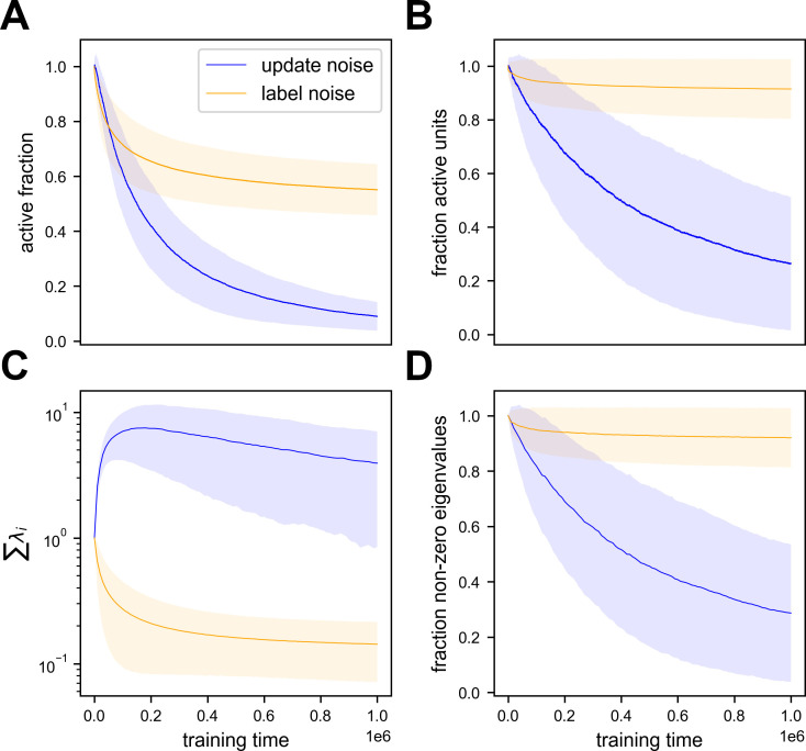
Recent studies show that, even in constant environments, the tuning of single neurons changes over time in a variety of brain regions. This representational drift has been suggested to be a consequence of continuous learning under noise, but its properties are still not fully understood. To investigate the underlying mechanism, we trained an artificial network on a simplified navigational task. The network quickly reached a state of high performance, and many units exhibited spatial tuning. We then continued training the network and noticed that the activity became sparser with time. Initial learning was orders of magnitude faster than ensuing sparsification. This sparsification is consistent with recent results in machine learning, in which networks slowly move within their solution space until they reach a flat area of the loss function. We analyzed four datasets from different labs, all demonstrating that CA1 neurons become sparser and more spatially informative with exposure to the same environment. We conclude that learning is divided into three overlapping phases: (i) Fast familiarity with the environment; (ii) slow implicit regularization; and (iii) a steady state of null drift. The variability in drift dynamics opens the possibility of inferring learning algorithms from observations of drift statistics.

Keywords: CA1; artificial neural network; mouse; neuroscience; noise; regularization; representational drift; theoretical neuroscience.

Figure 1.. Two types of possible movements within the solution space.

(A) Two options of how drift may look in the solution space. Random walk within the space of equally good solutions that is either undirected (left) or directed (right). (B) The qualitative consequence of the two movement types. For an undirected random walk, all properties of the solution will remain roughly constant (left). For the directed movement there should be a given property that is gradually increasing or decreasing (right).

Figure 2.. Continuous noisy learning leads to drift and spontaneous sparsification.

(A) Illustration of an agent in a corridor receiving high-dimensional visual input from the walls. (B) Loss as a function of training steps (log scale). Zero loss corresponds to a mean estimator. Note the rapid drop in loss at the beginning, after which it remains roughly constant. (C) Mean spatial information (SI, blue) and fraction of units with non-zero activation for at least one input (red) as a function of training steps. (D) Rate maps sampled at four different time points (columns). Maps in each row are sorted according to a different time point. Sorting is done based on the peak tuning value to the latent variable. (E) Correlation of rate maps between different time points along training. Only active units are used.

Figure 3.. Experimental data consistent with simulations.

Data from four different labs show sparsification of CA1 spatial code, along with an increase in the information of active cells. Values are normalized to the first recording session in each experiment. Error bars show standard error of the mean. (A) Fraction of place cells (slope=-0.0003 p < .001) and mean spatial information (SI) (slope=0.002, p < .001) per animal over 200 min (Khatib et al., 2023). (B) Number of cells per animal (slope=-0.052, p = .004) and mean SI (slope=0.094, p < .001) over all cells pooled together over 10 days. Note that we calculated the number of active cells rather than fraction of place cells because of the nature of the available data (Jercog et al., 2019b). (C) Fraction of place cells (slope=-0.048, p = .011) and mean SI per animal (slope=0.054, p < .001) over 11 days (Karlsson and Frank, 2008). (D) Fraction of place cells (slope=-0.026, p < .001) and mean SI (slope=0.068, p < .001) per animal over 8 days (Sheintuch et al., 2023).

Figure 4.. Generality of the results.

Summary of 616 simulations with various parameters, excluding stochastic gradient descent (SGD) with label noise (see Table 2). (A) Fraction of active units normalized by the first timestep for all simulations. Red line is the mean. Note that all simulations exhibit a stochastic decrease in the fraction of active units. See Figure 4—figure supplement 1 for further breakdown. (B) Dependence of sparseness (top) and sparsification time scale (bottom) on noise amplitude. Each point is one of 178 simulations with the same parameters except noise variance. (C) Learning a similarity matching task with Hebbian and anti-Hebbian learning using published code from Qin et al., 2023. Performance of the network (blue) and fraction of active units (red) as a function of training steps. Note that the loss axis does not start at zero, and the dynamic range is small. The background colors indicate which phase is dominant throughout learning (1 - red, 2 - yellow, 3 - green).

Figure 4—figure supplement 1.. Noisy learning leads to spontaneous sparsification.

Summary of 516 simulations with three different learning algorithms: Stochastic error descent (SED, Cauwenberghs, 1992), SGD, Adam. All values are normalized to the first time step of each simulation. The red lines indicate mean over all simulations. (A) Fraction active units – number of units with any response. (B) Active fraction – overall activity across all units (see methods).

Figure 5.. Noisy learning leads to a flat landscape.

(A) Gradient Descent dynamics over a two-dimensional loss function with a one-dimensional zero-loss manifold (colors from blue to yellow denote loss). Note that the loss is identically zero along the horizontal axis, but the left area is flatter. The orange trajectory begins at the red dot. Note the asymmetric extension into the left area. (B) Fraction of active units is highly correlated with the number of non-zero eigenvalues of the Hessian. (C) Update noise reduces small eigenvalues. Log of non-zero eigenvalues at two consecutive time points for learning with update noise. Note that eigenvalues do not correspond to one another when calculated at two different time points, and this plot demonstrates the change in their distribution rather than changes in eigenvalues corresponding to specific directions. The distribution of larger eigenvalues hardly changes, while the distribution of smaller eigenvalues is pushed to smaller values. (D) Label noise reduces the sum over eigenvalues. Same as (C), but for actual values instead of log.

Figure 5—figure supplement 1.. Label and update noise impose different regularization over the Hessian with distinct signatures in activity statistics.

Summary of 362 simulations with either label or update noise added to stochastic gradient descent (SGD) learning algorithm. All values are normalized to the first time step of each simulation. Lines indicate the mean of simulations and shaded regions indicate one standard deviation. Loss convergence varies between simulations, and is achieved on a scale of no more than 10⁵ time steps. (A) Active fraction as a function of training time. Note this metric decreases significantly for both types of noise. (B) Fraction of active units as a function of training time. For label noise, the change is much smaller. (C) Sum of the loss Hessian’s eigenvalues as a function of training time. Here the difference is apparent - label noise imposes slow implicit regularization over this metric while update noise does not. (D) Fraction of non-zero eigenvalues in the loss Hessian as a function of training time. As explained in the main text, update noise imposes implicit regularization over the sum of log-eigenvalues, which manifests as a zeroing of eigenvalues over time and thus a reduction in the fraction of active units.

Figure 6.. Illustration of sparsity metrics.

Author response image 1.. PV correlation between training time points averaged over 362 simulations.

(B) Mean SI of units normalized to first time step, averaged over 362 simulations. Red line shows the average time point of loss convergence, the shaded area represents one standard deviation.

References

-
- Aviv-Ratzon Driftreg. swh:1:rev:cb83d928b66401405c26500ab93b4b98ef7b3b67Software Heritage. 2024 https://archive.softwareheritage.org/swh:1:dir:b6b2c3944401b7c73209f6d47...
- Bengio Y, Lee DH, Bornschein J, Mesnard T, Lin Z. Towards Biologically Plausible Deep Learning. arXiv. 2015 https://arxiv.org/abs/1502.04156
- Blanc G, Gupta N, Valiant G, Valiant P. Implicit regularization for deep neural networks driven by an ornstein-uhlenbeck like process. Conference on learning theory.2020.
Publication types
MeSH terms
Grants and funding
LinkOut - more resources
Full Text Sources
Miscellaneous