A Perspective on Protein Structure Prediction Using Quantum Computers

Abstract

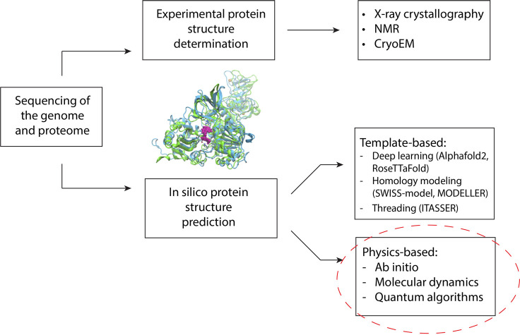
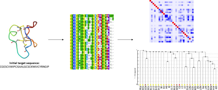
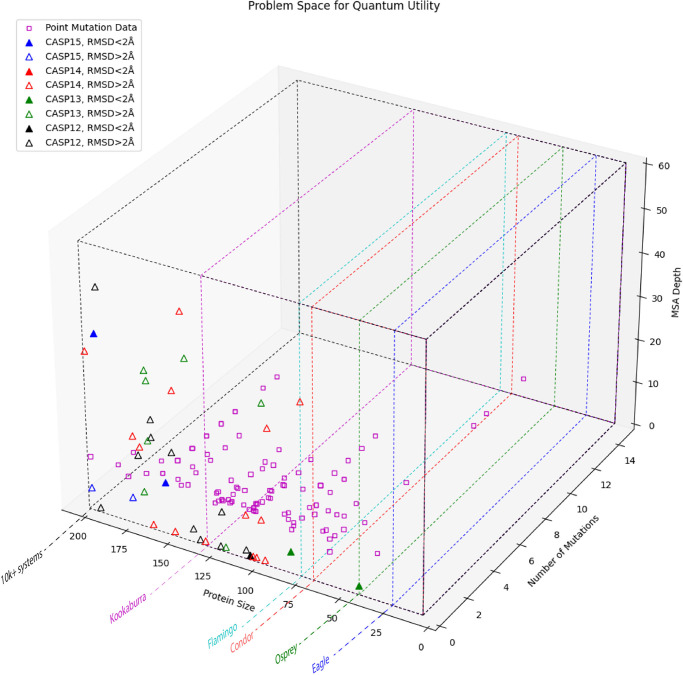
Despite the recent advancements by deep learning methods such as AlphaFold2, in silico protein structure prediction remains a challenging problem in biomedical research. With the rapid evolution of quantum computing, it is natural to ask whether quantum computers can offer some meaningful benefits for approaching this problem. Yet, identifying specific problem instances amenable to quantum advantage and estimating the quantum resources required are equally challenging tasks. Here, we share our perspective on how to create a framework for systematically selecting protein structure prediction problems that are amenable for quantum advantage, and estimate quantum resources for such problems on a utility-scale quantum computer. As a proof-of-concept, we validate our problem selection framework by accurately predicting the structure of a catalytic loop of the Zika Virus NS3 Helicase, on quantum hardware.

Figure 1

Overview of the PSP pipeline. Following genomic sequencing, the primary amino acid sequence is determined. The experimental method then starts with expressing this protein by genetically modifying another organism with this new sequence. This organism will then translate these proteins, and the new protein of interest can be isolated, purified, and then solved using X-ray crystallography, NMR, or CryoEM. The in silico methods on the other hand, simply take the primary amino acid sequence as input and the structure is predicted by either a physics-based method (where the underlying biophysics is somehow simulated) or a template-based method (where machine learning algorithms predict structures based on patterns found in a training set of experimental templates). The method we adopt in this work falls under the category of physics-based algorithms. As an illustrated example, an in silico model and X-ray crystal structure of the SARS-CoV2 NSP13 helicase (PDB: 7NN0) are superimposed, along with a docked known inhibitor (colored in magenta).

Figure 2

This graphic was originally created and released in the public domain by Ken A. Dill. Original caption: The illustrations of proposed energy landscape that each demonstrate the degree of freedom a protein possesses in terms of configurations and the multidimensional routes that a protein can take to achieve its final configuration. From left to right for proposed funnel-shaped energy landscape: the idealized smooth funnel, the rugged funnel, the Moat funnel, and the Champagne Glass funnel.

Figure 3

A graphical representation of the rapid growth in the search space as a function of n amino acids. (a) The data considers that for a protein with n amino acids, there are n – 1 peptide bonds. For each peptide bond, there are also 2 other bond angles on either side of the α carbon, ϕ and ψ, and assumes that each peptide in the sequence can adopt up to 3 conformations (3 combinations of these bond angles). (b) So, for a protein with n amino acids, there are a total of 3^2(n–1) possible conformations. Assuming 1 ps is spent to sample each conformation, the y-axis represents the total exploration time in years to sample all possible conformations for a protein with n amino acids. For a detailed discussion on Levinthal’s paradox and growth in the conformational search space, please see Section 2 of the Supporting Information.

Figure 4

Free energy landscapes of (a) TC10b and (b) TC5b derived from molecular dynamics simulations at their melting points of 329 and 315 K, respectively. The folded NMR structures are quite similar (0.8 Å RMSD between them), but the free energy landscape is dramatically different, with TC10b demonstrating two possible folding pathways and their minima, as opposed to the more well-defined funnel and obvious global minimum in the case of TC5b. The three point mutations between these structures give rise to different physicochemical properties such as their melting temperatures, and accordingly different free energy landscapes.

Figure 5

(a) The common anatomy of transmembrane proteins like the G-protein coupled receptor (GPCR) superfamily. (b) The incomplete experimentally determined crystal structure of H3HR, which is essentially missing the entire ICD. (c) Alignment and comparison between the experimental structure and computational models of H3HR, highlighting the excellent agreement in the TM region, but the significant discrepancies in the predicted ICD. (d) A detailed comparison of the structures reveals that the TM region is closely modeled with RMSDs of 0.2 to 4.9 Å, while the ICD varies drastically with RMSDs of 13.8 to 26.8 Å. The least accurate model is arguably AlphaFold2’s, with a highly disordered ICD and an extended C- and N-terminus.

Figure 6

A typical MSA generation pipeline to extract statistical summaries. After the sequences are aligned, the covariance matrix and the phylogenetic tree are constructed to capture coevolutionary information.

Figure 7

The plots highlight the performance of all groups for the target proteins, however we further distinguish: (a) Performance of versions of AlphaFold2 that participated in CASP15 for the three targets. (b) Performance of top three ranked groups with respect to overall z-scores in CASP15 for the three targets. The graphs show the percentage of residues in the target protein that are under a certain distance cutoff. It is easy to see that for the target protein T1122, no group was able to predict all residues under 10 Å. For T1160 and T1161, which exhibit point mutations, deep learning-based methods used by the groups listed has 80% of residues under 10 Å. In general, sharper increasing curves indicate poorer predictions. Images generated from CASP15 official Web site from the results.

Figure 8

Subspace of PSP problems partitioned with different color rectangular boxes. This is in parallel with the IBM Quantum hardware roadmap as system size increases in terms of qubits. The nested rectangular boxes represent the subset of proteins where deep learning based methods are known to perform poorly (data point markers with no facecolors), hence other ab initio methods, including quantum algorithms, can potentially yield better predictions. CASP data is obtained from, however sequence length data is added from CASP website directly. For each protein on the plot, average RMSD from the top 10% of the groups is calculated and added to the data. Point mutation data is obtained from, and the MSA depth (N_eff) values are calculated using HHblits and HHpred tools. Average RMSD values are not calculated for point mutation data set since they are not CASP targets. Clearly, there are many more proteins within these boxes. Our goal is to show that there are nontrivial, high-value targets for each of these regimes. The alignment with the IBM Quantum Roadmap is more of a symbolic representation. While we estimated qubit costs for the problem instances, one needs to perform a rigorous resource estimation for a concrete representation. This is beyond the scope of this work. We assume that for any range of qubit number, the quantum computer is able to perform a reasonable number of gate operations under reasonable time frame.

Figure 9

A schematic representation of the workflow used in this study. The most computationally demanding part, finding a coarse-grain representation of the lowest energy conformation of the protein structure, is performed on a quantum computer. The following steps are handled classically to convert the output into a desired format and postprocess to construct the full structure, while preserving the quantum algorithm’s originally predicted backbone geometry from the coarse grain model. A final refinement of the all-atom structure is then performed through further energy minimization using a molecular mechanics force field. This last step allows the protein to potentially reach an even more optimal configuration as the atoms and bonds are no longer constrained to the four turns of the original lattice structure.

Figure 10

An initial validation of the workflow with the Zika virus helicase P-loop (LHPGAGK). In all cases, the coordinates from the experimental crystal structure are colored in cyan. The lowest RMSD relative to the experimental structure is achieved by (a) PEP-FOLD3, followed very closely by (b) the quantum algorithm executed on IBM_Cleveland, and then by (c) the problem Hamiltonian solved classically by brute force and the QUBO Hamiltonian solved by a classical mixed-integer linear solver (both approaches yielded the same solution). The least accurate model was produced by (d) AlphaFold2. This is observed by the relative RMSD values in each case, as well as (f) the measured radius of gyration Rg. The conformational energy plot in (e) appears to demonstrate that VQE begins to continuously sample conformations around the basin after a handful of VQE iterations. Note: while these residues are numbered 1–7 here, they correspond to 194–200 in the crystal structure, PDB: 5gjb.

Figure 11

(a) The total number of qubits scale quadratically as the protein size increases. We consider both configuration and interaction qubits to encode a given amino acid sequence, and analyze the scaling. (b) We estimate an upper bound for the number of measurements needed to predict a protein structure within a fixed energy error margin using the work from. The energy unit is converted to kcal/mol from Hartree for consistency with our workflow. See Section 5.4 of the Supporting Information for mathematical formula to calculate the upper bound. The three plots show different upper limits to predict a protein structure within ε = 1, 5, 10 kcal/mol range of the lowest energy conformation. The upper bound is not known to be tight. We further expect the empirically sufficient number of measurements to be significantly lower than this upper bound. (c) Shows the total number of ECR gates in the circuit as the protein size increases for different optimization levels. Qiskit transpiler allows four levels of optimization which are defined in. (d) Shows the ECR-depth as a function of protein size.

References

1. Dill K. A.; Ozkan S. B.; Shell M. S.; Weikl T. R. Annu. Rev. Biophys. 2008, 37, 289–316. 10.1146/annurev.biophys.37.092707.153558. - DOI - PMC - PubMed
1. Dill K. A.; MacCallum J. L. Science 2012, 338, 1042–1046. 10.1126/science.1219021. - DOI - PubMed
1. Jumper J.; Evans R.; Pritzel A.; Green T.; Figurnov M.; Ronneberger O.; Tunyasuvunakool K.; Bates R.; Žídek A.; Potapenko A.; et al. Nature 2021, 596, 583–589. 10.1038/s41586-021-03819-2. - DOI - PMC - PubMed
1. Baek M.; DiMaio F.; Anishchenko I.; Dauparas J.; Ovchinnikov S.; Lee G. R.; Wang J.; Cong Q.; Kinch L. N.; Schaeffer R. D.; et al. Science 2021, 373, 871–876. 10.1126/science.abj8754. - DOI - PMC - PubMed
1. Zhou X.; Zheng W.; Li Y.; Pearce R.; Zhang C.; Bell E. W.; Zhang G.; Zhang Y. Nat. Protoc. 2022, 17, 2326–2353. 10.1038/s41596-022-00728-0. - DOI - PubMed
LinkOut - more resources