Disentangling signal and noise in neural responses through generative modeling

Abstract

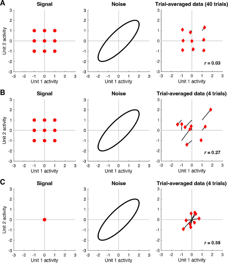
Measurements of neural responses to identically repeated experimental events often exhibit large amounts of variability. This noise is distinct from signal, operationally defined as the average expected response across repeated trials for each given event. Accurately distinguishing signal from noise is important, as each is a target that is worthy of study (many believe noise reflects important aspects of brain function) and it is important not to confuse one for the other. Here, we describe a principled modeling approach in which response measurements are explicitly modeled as the sum of samples from multivariate signal and noise distributions. In our proposed method-termed Generative Modeling of Signal and Noise (GSN)-the signal distribution is estimated by subtracting the estimated noise distribution from the estimated data distribution. Importantly, GSN improves estimates of the signal distribution, but does not provide improved estimates of responses to individual events. We validate GSN using ground-truth simulations and show that it compares favorably with related methods. We also demonstrate the application of GSN to empirical fMRI data to illustrate a simple consequence of GSN: by disentangling signal and noise components in neural responses, GSN denoises principal components analysis and improves estimates of dimensionality. We end by discussing other situations that may benefit from GSN's characterization of signal and noise, such as estimation of noise ceilings for computational models of neural activity. A code toolbox for GSN is provided with both MATLAB and Python implementations.

Figure 1.. Trial averaging is insufficient for removing the effects of noise.

Here we perform simulations to illustrate how noise correlations persist after trial averaging (code available at https://osf.io/fc589). A, In this simulation, responses to 9 conditions are measured from 2 units. The left shows the signal, i.e. responses in the absence of noise. The middle shows the noise, i.e. trial-to-trial response variability for a fixed condition; the noise is drawn from a zero-mean multivariate Gaussian distribution (ellipse indicates a Mahalanobis distance of 2). The right shows responses averaged across 40 trials for each condition (black lines join the trial average to the corresponding signal). B, Same as panel A except that 4 trials per condition are used. C, Same as panel B except that the signals associated with the 9 conditions are all set to zero.

Figure 2.. Schematic of GSN.

Here we depict an example involving $n=2$ units, $c=40$ conditions, and $t=3$ trials per condition (code available at https://osf.io/7k2m5). In each plot, the black cross and black ellipse indicate the mean and spread (Mahalanobis distance of 2) of a multivariate Gaussian distribution. For definitions of symbols, please see Methods. A, Signal. The signal indicates responses to different conditions in the absence of noise and is modeled as a multivariate distribution. B, Noise. The noise indicates trial-to-trial variability for a given condition and is modeled as a zero-mean multivariate distribution. C, Data. The data are modeled as the sum of a sample from the signal distribution and a sample from the noise distribution. D, Estimate of data distribution. Given a set of measured responses, we compute trial-averaged responses and estimate the mean and covariance of these responses, yielding the estimate of the data distribution. E, Estimate of noise distribution. We compute the covariance of responses to each condition and average across conditions, yielding the estimate of the noise distribution. F, Estimate of signal distribution. We subtract the estimated parameters of the noise distribution from the estimated parameters of the data distribution, yielding the estimate of the signal distribution.

Figure 3.. Estimation of signal and noise distributions.

Here we show results of simulations that assess how well GSN estimates the signal and noise distributions that underlie a set of measurements (code available at https://osf.io/5uskr). All simulations involve 10 units whose responses are generated as the sum of a sample from a signal distribution and a sample from a noise distribution. Both distributions are multivariate Gaussian with zero mean but have different covariances (as depicted). For different combinations of number of conditions (samples from the signal distribution) and number of trials (samples from the noise distribution for each condition), we perform 1,000 simulations. In each simulation, we generate responses and analyze the resulting data using three different methods: ‘Naive’ refers to simple heuristic methods for estimating signal and noise covariance (see main text), ‘No shrinkage’ is the GSN method with standard covariance estimation, and ‘Shrinkage’ is the GSN method with shrinkage-based covariance estimation. Blue number labels highlight specific aspects of the results that are discussed in the main text. A–C, Detailed inspection of results for specific condition and trial numbers. In the scatter plots, purple and brown dots indicate diagonal and off-diagonal elements of the covariance matrix, respectively, and error bars indicate standard deviation across simulations. At the far right are plots of the eigenspectra (mean across simulations) produced by the three methods, as well as the ground-truth eigenspectra.

Figure 4.. Ground-truth recovery of covariance.

Here we quantify how well different methods recover signal and noise covariance (code available at https://osf.io/5uskr and https://osf.io/3yvtg). Performance is quantified using coefficient of determination $\left(R^2\right)$ with respect to values in the upper triangle of the covariance matrix (including the diagonal). The ‘Split-half’ method involves computing covariance across independent splits (trials) of the data. A–B, Recovery performance for the simple scenario illustrated in Figure 3. We vary the number of trials while holding the number of conditions fixed at 50 (panel A), and we vary the number of conditions while holding the number of trials fixed at 5 (panel B). Markers indicate the mean across 1,000 simulations. C, Recovery performance for a set of scenarios in which the number of units is varied (rows) and the dimensionality of the signal and noise is varied (columns). In these scenarios, signal and noise eigenspectra are governed by the power-law function $d^{-\alpha }$ where $d$ is the 1-indexed dimension number and $\alpha$ is an exponent parameter. We fix the number of trials at 5 and vary the number of conditions. Markers indicate the mean across 50 simulations.

Figure 5.. Ground-truth recovery of effective dimensionality and power-law exponent.

Here we quantify how well different methods recover two summary metrics of signal and noise eigenspectra: effective dimensionality and power-law exponent (code available at https://osf.io/3yvtg). Recovery performance is plotted for the same scenarios shown in Figure 4C. The cvPCA method estimates the signal eigenspectrum by projecting two splits of a given set of data onto principal components (PCs) and calculating the dot product between the two sets of projections obtained for each PC. The MEME method estimates the signal eigenspectrum by estimating signal eigenmoments from a given set of data and then adjusting the parameters of an eigenspectrum model to match the estimated eigenmoments. Markers indicate the mean across 50 simulations, and the horizontal dotted line indicates the ground-truth value. Note that the Split-half, cvPCA, and MEME methods do not provide estimates for the noise (and are therefore not plotted).

Figure 6.. Application of GSN to example fMRI data.

Here we demonstrate the application of GSN to example data from FFA-1 (330 vertices × 10,000 images × 3 trials) (code available at https://osf.io/yxrsp). A, Signal and noise covariance estimates. In addition to GSN outputs (first and second columns), we show results from naive estimation of signal covariance which involves simply calculating the covariance of trial-averaged data (third column). B, Results for shuffled data. As a control, we shuffled responses across all images and trials and reanalyzed the data. C, Conversion to correlation units. The results of panel A are re-plotted after converting covariance to correlation units. D, Estimates as a function of amount of data. We varied the fraction of images to which GSN is applied (e.g. 1/16 corresponds to 625 of 10,000 images being used). This was done such that data subsets were mutually exclusive of one another.

Figure 7.. GSN disentangles signal and noise in principal components analysis (PCA).

Here we use PCA to analyze the results of GSN as applied to FFA-1 (code available at https://osf.io/f34bc). A, Eigenspectra. For each of the eight participants (P1–P8), we plot the eigenspectra of the signal and noise as estimated by GSN (‘Signal (GSN)’, ‘Noise (GSN)’), as well as the eigenspectrum of the trial-averaged data (‘Naive’). The main plots show results on a linear scale for up to the first 10 dimensions; the insets show results on a base-10 log-log scale for up to the first 100 dimensions. Numbers above each main plot indicate the effective dimensionality of the three eigenspectra. B, Split-half reliability of principal components. The cosine similarity between corresponding principal components from two split-halves of the data from each participant is plotted for up to the first 100 dimensions. The thick black line indicates the mean across participants. C, Across-participant consistency. A common set of 515 images were viewed three times each by all participants. For each participant, we computed the projections of trial-averaged responses to these 515 images onto either (i) the first principal component of the covariance of the trial-averaged data (‘Standard PCA’) or (ii) the first principal component of the signal covariance estimated by GSN (‘GSN PCA’). The cosine similarity of these projections between each pair of participants is shown.

References

1. Allen E.J., St-Yves G., Wu Y., Breedlove J.L., Prince J.S., Dowdle L.T., Nau M., Caron B., Pestilli F., Charest I., Hutchinson J.B., Naselaris T., Kay K., 2022. A massive 7T fMRI dataset to bridge cognitive neuroscience and artificial intelligence. Nat. Neurosci. 25, 116–126. - PubMed
1. Averbeck B.B., Latham P.E., Pouget A., 2006. Neural correlations, population coding and computation. Nat. Rev. Neurosci. 7, 358–366. - PubMed
1. Azeredo da Silveira R., Rieke F., 2021. The geometry of information coding in correlated neural populations. Annu. Rev. Neurosci. 44, 403–424. - PubMed
1. Bays P.M., 2014. Noise in neural populations accounts for errors in working memory. J. Neurosci. 34, 3632–3645. - PMC - PubMed
1. Bickel P.J., Levina E., 2008a. Regularized estimation of large covariance matrices. Ann. Stat. 36, 199–227.
Publication types