Theta oscillons in behaving rats

Abstract

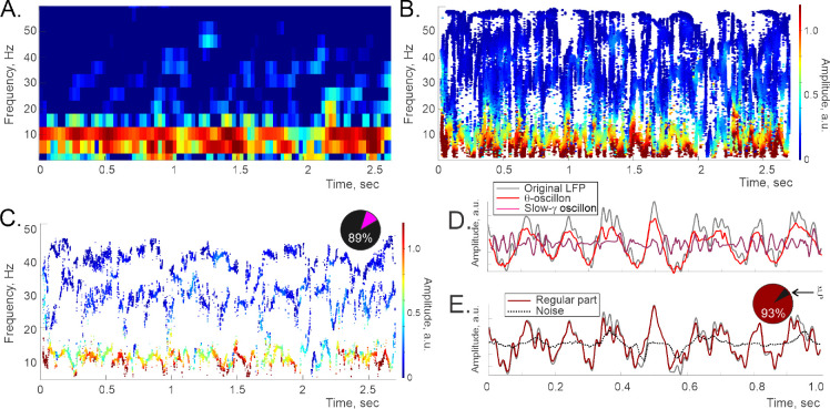
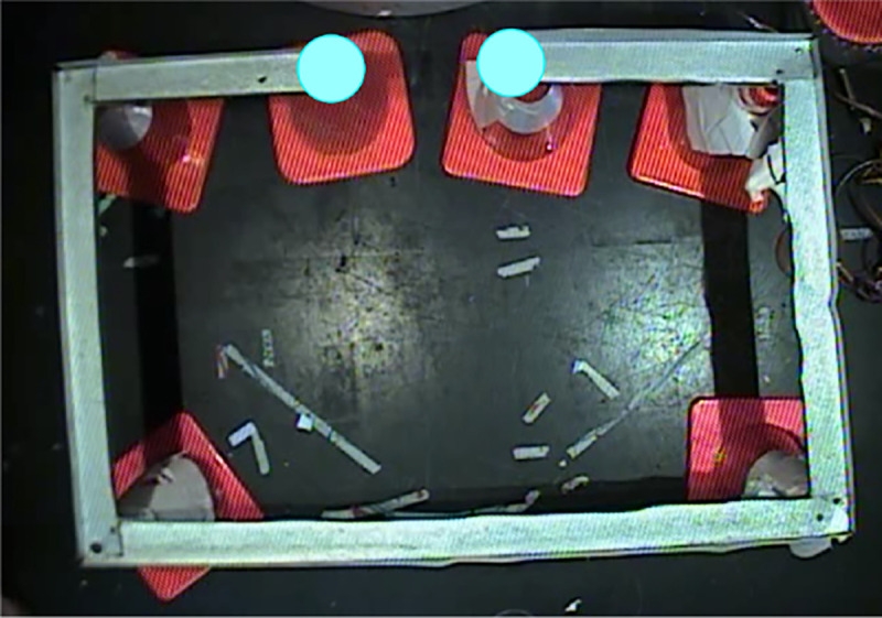
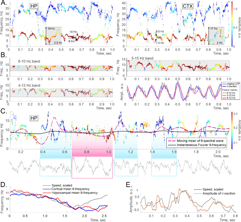
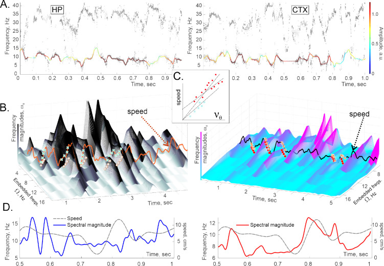
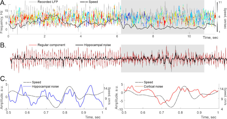
Recently discovered constituents of the brain waves-the oscillons-provide high-resolution representation of the extracellular field dynamics. Here we study the most robust, highest-amplitude oscillons that manifest in actively behaving rats and generally correspond to the traditional $\theta$ -waves. We show that the resemblances between $\theta$ -oscillons and the conventional $\theta$ -waves apply to the ballpark characteristics-mean frequencies, amplitudes, and bandwidths. In addition, both hippocampal and cortical oscillons exhibit a number of intricate, behavior-attuned, transient properties that suggest a new vantage point for understanding the $\theta$ -rhythms' structure, origins and functions. We demonstrate that oscillons are frequency-modulated waves, with speed-controlled parameters, embedded into a noise background. We also use a basic model of neuronal synchronization to contextualize and to interpret the observed phenomena. In particular, we argue that the synchronicity level in physiological networks is fairly weak and modulated by the animal's locomotion.

FIG. 1.

Oscillons and spectral waves constructed for the LFP data recorded in the rat’s cortex. A. Fourier spectrogram: the high-power stripe between about 4 and 12 Hz marks the conventional $\theta$-band, the slow-$\gamma$ domain lays approximately between 20 and 45 Hz. B. The corresponding full Padé spectrogram, same time resolution, shows the pattern of “flexible” frequencies, both stable and unstable. The vertical position of each dot marks a specific frequency value, the horizontal position marks the corresponding time, and the color indicates the instantaneous amplitude (colorbar on the right). C. Most frequencies, (typically over 80%, dark section on the pie diagram), are unstable or “noise-carrying.” Removing them reveals the regular Padé spectrogram, on which the stable frequencies trace out regular timelines—spectral waves, $v_q\left(t\right)$. Color change along each spectral wave encodes the corresponding time-dependent amplitude, $A_q\left(t\right)$ (Eq. 1). D. Combining a particular spectral wave, $v_q\left(t\right)$, with its amplitude, $A_q\left(t\right)$, yields an individual oscillon, as indicated by Equation 1). Shown is a one-second-long segment of the cortical $\theta$-oscillon (red trace) and the slow-$\gamma$ oscillon (pink trace). Notice that summing just these two oscillons (first two terms in the Eq. 2) already approximates the full LFP profile (gray line) quite closely. E. The superposition of all the inputs with regular frequencies (dark red trace), closely matches the amplitude original signal (gray trace). The difference is due to the noise component, $\xi \left(t\right)$, carried by the unstable frequencies (dotted black line) typically accounts for less than 5−7% of the signal’s net power during active behaviors (dark section on the pie diagram), and about 10−15% during quiescence. Data sampled in a 6 months old, wake male rat during active behavior.

FIG. 2.

Linear track explored by the rat is 3.5 meters long, a typical run between the food wells (blue dots) takes about 30 sec. Fast moves over the straight segments last 5 − 6 secs, slowdowns occur at the corners and during feeding.

FIG. 3.

A. The lowest spectral wave occupies the domain that is generally attributed to the $\theta$-frequency band. The color of each dot represents the amplitude, as on Fig. 1. The spectral widths range from about 17 to about 2 Hz (gray boxes). B. The hippocampal $\theta$-oscillon’s spectral wave, made visible through three “frequency slits” that represent three most commonly used $\theta$-bands, 4–12 Hz, 5–15 Hz, and 6–11 Hz (gray stripes). The frequencies that fit into a slit are the ones that produce the corresponding Fourier wave, shown as red-shaded traces on the bottom right panel. Note that the spectral waves are crosscut by all $\theta$-bands. The Fourier waves are close to each other (DTW distances $D(f_{{\theta }_1}^h,f_{{\theta }_2}^h)\approx 6\mathrm{\%},D(f_{{\theta }_2}^h,f_{{\theta }_3}^h)\approx 5\mathrm{\%},D(f_{{\theta }_3}^h,f_{{\theta }_1}^h)\approx 8\mathrm{\%})$, but further from the $\theta$-oscillon (e.g., $D({\vartheta }_{\theta }^h,f_{{\theta }_2}^h)\approx 9\mathrm{\%})$, which, in turn, is closer to the original LFP (the $l\left(t\right)$ in Eq. 2, gray trace, $(D({\ell }^h,{\vartheta }_{\theta }^h)=4\mathrm{\%})$. C. A longer segment of a hippocampal-$\theta$ spectral wave. The nearly-constant solid black trace in the middle shows the instantaneous Fourier $\theta$-frequency. The dashed purple line shows the spectral wave’s moving average, which clearly provides a more detailed description of the $\theta$-rhythm’s trend. The waveform (bottom panel) is regular when the mean is steady (pink box), and corrugates when the mean is perturbed (blue boxes). D. The moving mean of the hippocampal and cortical $\theta$-oscillons’ spectral waves (blue and red curves respectively) follow the speed profile (dashed gray curve). The latter was scaled vertically to match, for illustrative purposes, see also Fig. S4. E. The amplitude of the hippocampal $\theta$-oscillon also co-varies with the speed, which was captured previously via Fourier analyses [31, 34, 35].

FIG. 4.. Spectral waves and embedded frequencies.

A. The spectral patterns produced via shifting-window evaluation of instantaneous frequencies are intermittent (Fig. 3A). To recapture the underlying continuous spectral dynamics, we interpolated the raw datapoints over a uniform time series, thus recovering the hippocampal (left) and the cortical (right) spectral waves with uninterrupted shapes. B. The contiguous data series allow constructing 3D Welch’s spectrogram on which each peak along the frequency axis highlights a particular embedded frequency. Altitudinal shadowing emphasizes higher peaks (colorbar along the vertical axis). Note that most peaks in both hippocampal (left) and the cortical (right) $W$-spectrograms are localized not only in frequency but also in time, indicating short-lived perturbations of spectra. The dynamics of these frequencies is coupled with the speed—higher speeds drive up the magnitudes of the embedded frequencies. The speed profile is scaled vertically and shifted horizontally to best match the frequency magnitudes (orange and black trace respectively). While the response of the hippocampal frequency to speed is nearly immediate (about $\tau =70-120\text{ms}$ delay), the cortical response is delayed by about $\tau =300\pm 50\text{s}$. C. Examples of the individual cortical peaks’ magnitudes, sampled at random, over particular frequencies (heights of the dots on the panels B) and the corresponding speeds (heights of the crosses) exhibit clear quasi-linear dependencies. The exponents of these dependencies may slightly change from one appearance of a peak (an instantiation of an embedded frequency) to another. D. The net magnitude of the spectral wave ($\theta$-bandwidth) co-varies with the speed with the delay of $=100\mathrm{m}\mathrm{s}$, depending on the case, in the hippocampus (left panel) and an extra $\tau =300\mathrm{m}\mathrm{s}$ in the cortex (right panel).

FIG. 5.. Spectral wave magnitude, noise and speed.

A. A segment of a hippocampal spectral wave shows magnitude increase during activity with speed, which reflects increased level of synchronization (see below). Shaded area highlights a period of slow motion, during which the noise escalates. The original LFP amplitude is shown by the gray trace in the background, for reference. The dashed black curve shows the animal’s speed. B. The dynamics of the regular part of the LFP (red trace) and the noise component (dotted black trace), obtained for a 12-second lap. Original LFP is shown by gray trace in the background. C. The hippocampal (left panel) and cortical (right panel) noise levels follow speed, but more loosely than the oscillon’s amplitude.

FIG. 6.. Kuramoto model.

1000 oscillators (phasors) with base frequencies normally distributed around 8 Hz with the variance 1 Hz, coupled via equation 7, produce a mean field characterized by a single spectral wave—a solitary Kuramoto oscillon (gray trace in the background, scaled up on the top panel 10 times for visibility). On all panels, the maximal amplitude defines the color scale. A. At small couplings, $K$-oscillon has low amplitude $\left(A_K\preccurlyeq 0.02A_{\mathrm{m}\mathrm{a}\mathrm{x}}\right)$ and often reshapes (the spectral wave then disrupts, blue boxes). The $W$-spectrogram (right panel) shows that the embedded frequencies restructure at ~ 100 ms timescale. B. As the coupling between phasors grows, the synchronized amplitude builds up and the $K$-oscillon’s shape regularizes. Note that when the spectral wave flattens out, the oscillon is nearly sinusoidal (strong synchronization, brown boxes), and the dynamics of the embedded frequencies during these periods are suppressed (right panel). C. At large couplings, synchronization becomes persistent: the spectral wave narrows, the embedded frequencies die out and the oscillon reduces to a nearly-sinusoidal harmonic. D. A hippocampal $\theta$-oscillon regularizes its spectral wave and yields higher amplitude when the rat’s speed is steady (gray dashed line, shifted by 80 ms); desynchronization occurs when the speed is low or transient. E. The oscillon’s amplitude, $A_K$(orange curve), the magnitude of its spectral wave (purple curve), and the noise level, $\xi$ (gray curve), for different coupling strengths. As the system synchronizes $(1.7\lesssim \lambda \precsim 3$, the amplitude grows, while the spectral undulations and the noise subdue. At higher couplings noise is suppressed and regular wave dominates.

References

1. Buzsáki G., Anastassiou C. & Koch C. The origin of extracellular fields and currents—EEG, ECoG, LFP and spikes. Nat. Rev. Neurosci. 13: 407–402 (2012). - PMC - PubMed
1. Buzsáki G. Rhythms in the brain. Oxford University Press, USA, (2011).
1. Colgin L. Rhythms of the hippocampal network. Nat. Rev. Neurosci. 17: 239–249 (2016). - PMC - PubMed
1. Thut G. Miniussi C. & Gross J. The Functional Importance of Rhythmic Activity in the Brain. Current Biology 22: R658 (2012). - PubMed
1. Kopell N., Kramer M., Malerba P. & Whittington M. Are different rhythms good for different functions? Front. Human Neurosci., 4: 187 (2010). - PMC - PubMed
Publication types