Genome organization around nuclear speckles drives mRNA splicing efficiency

Abstract

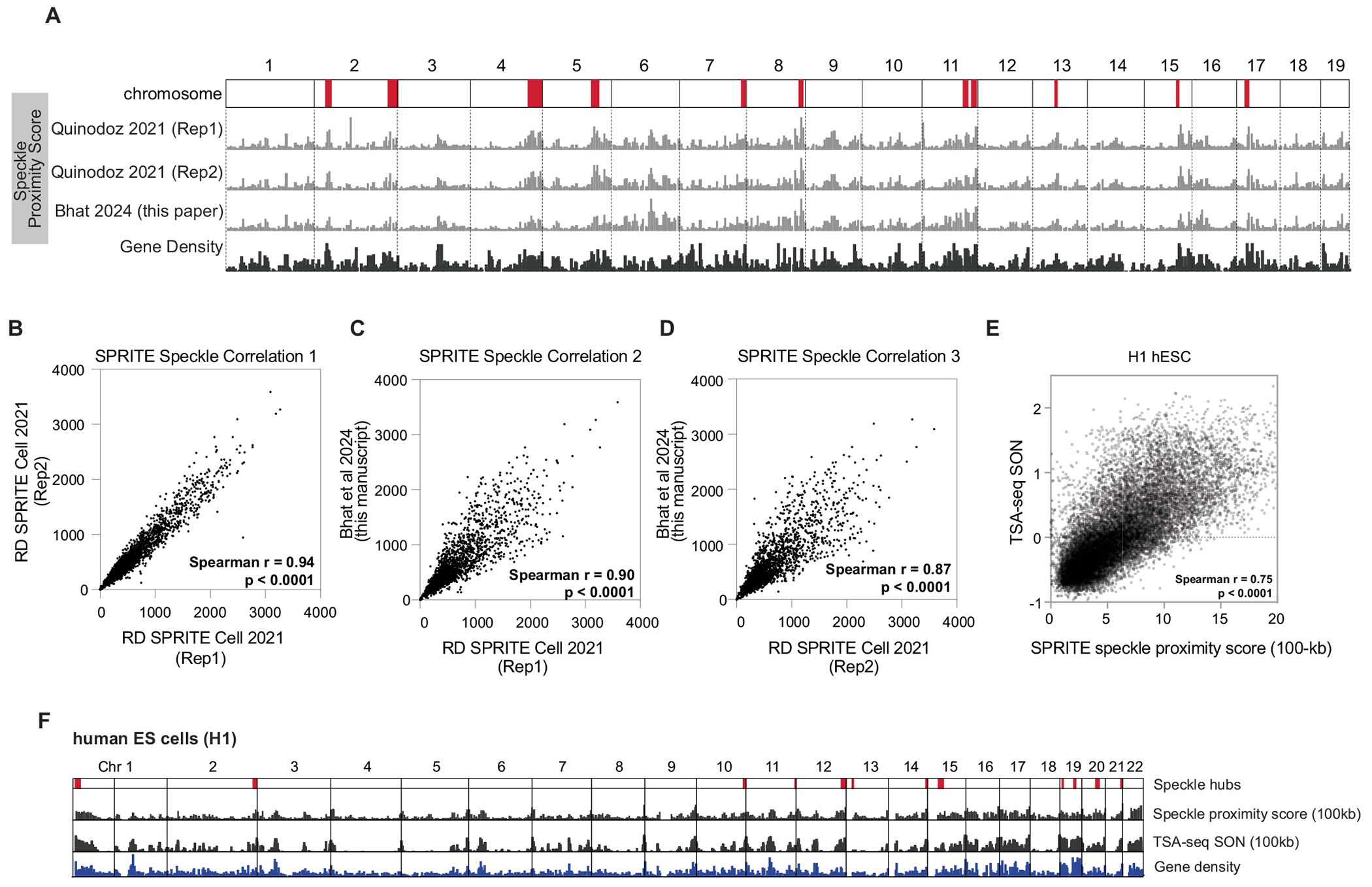
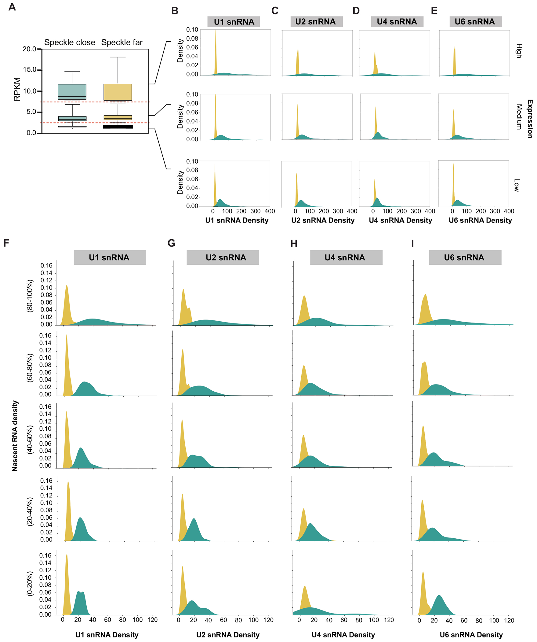
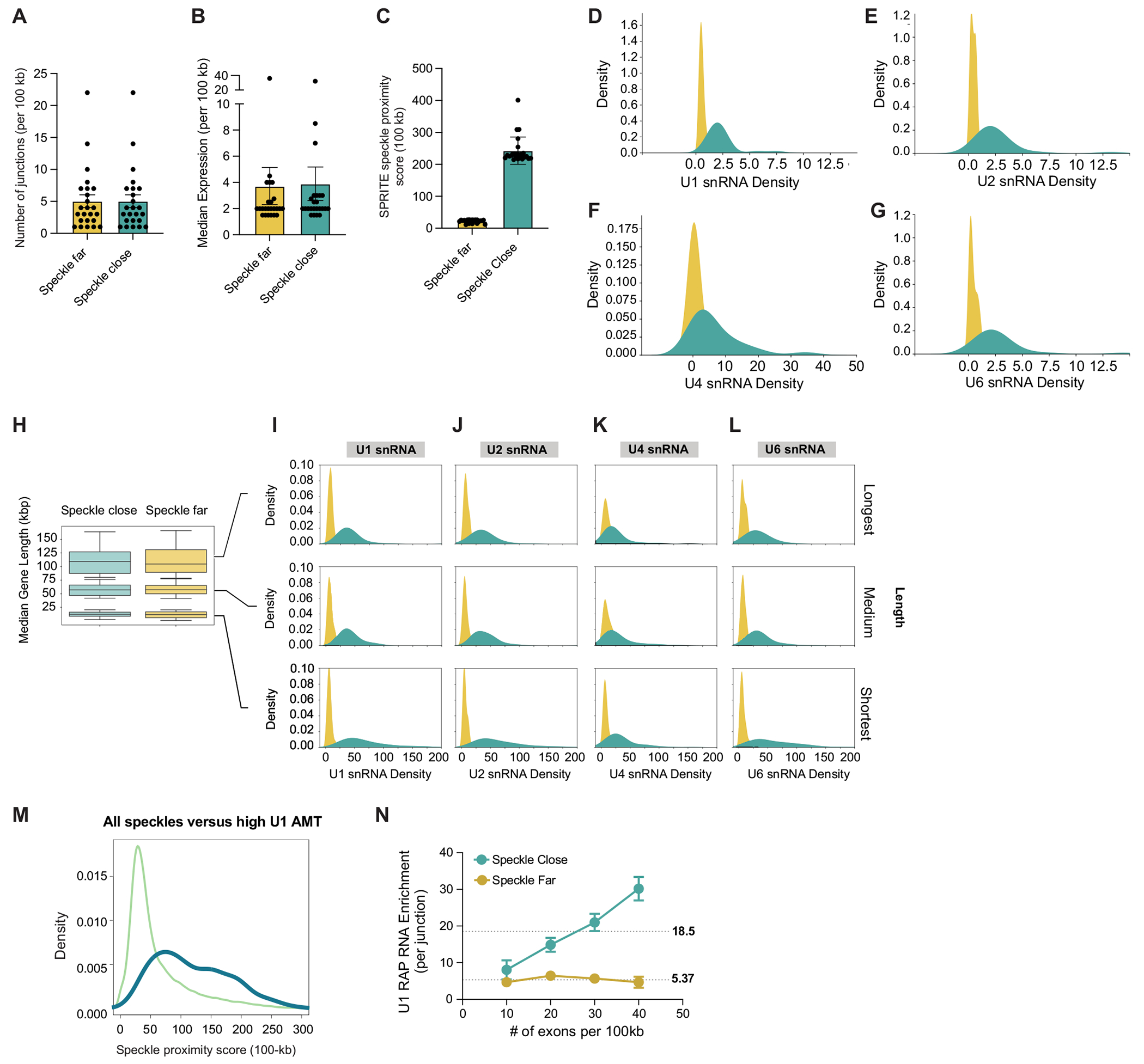
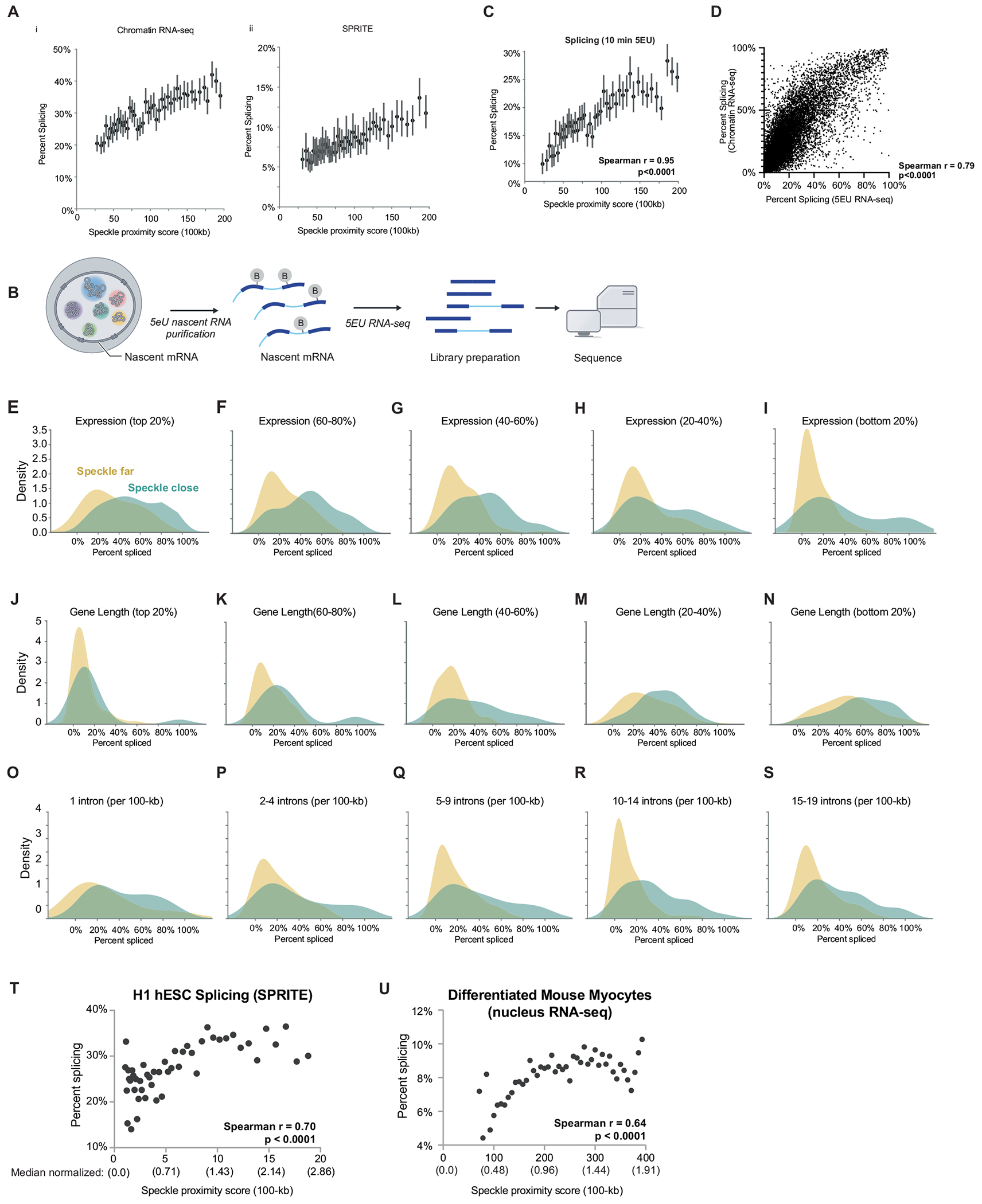
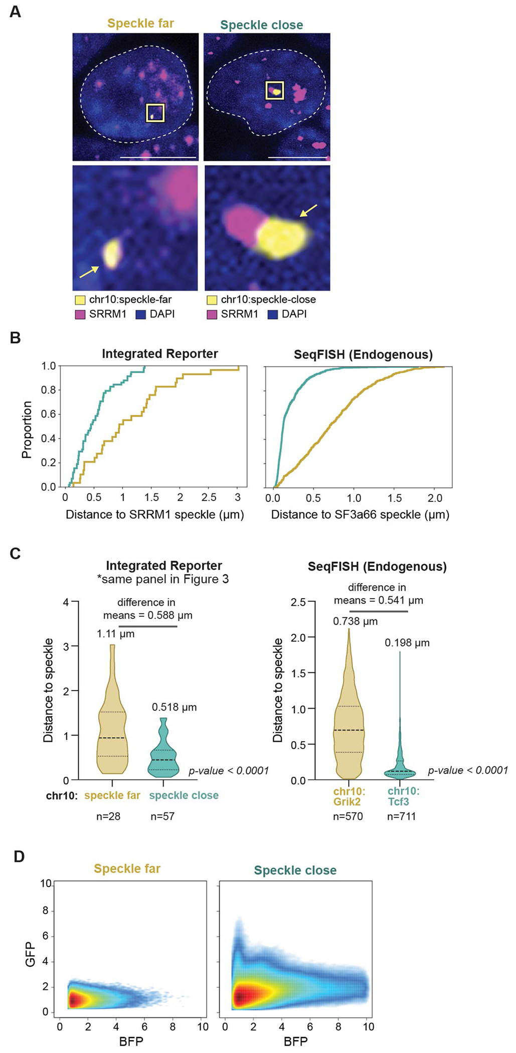
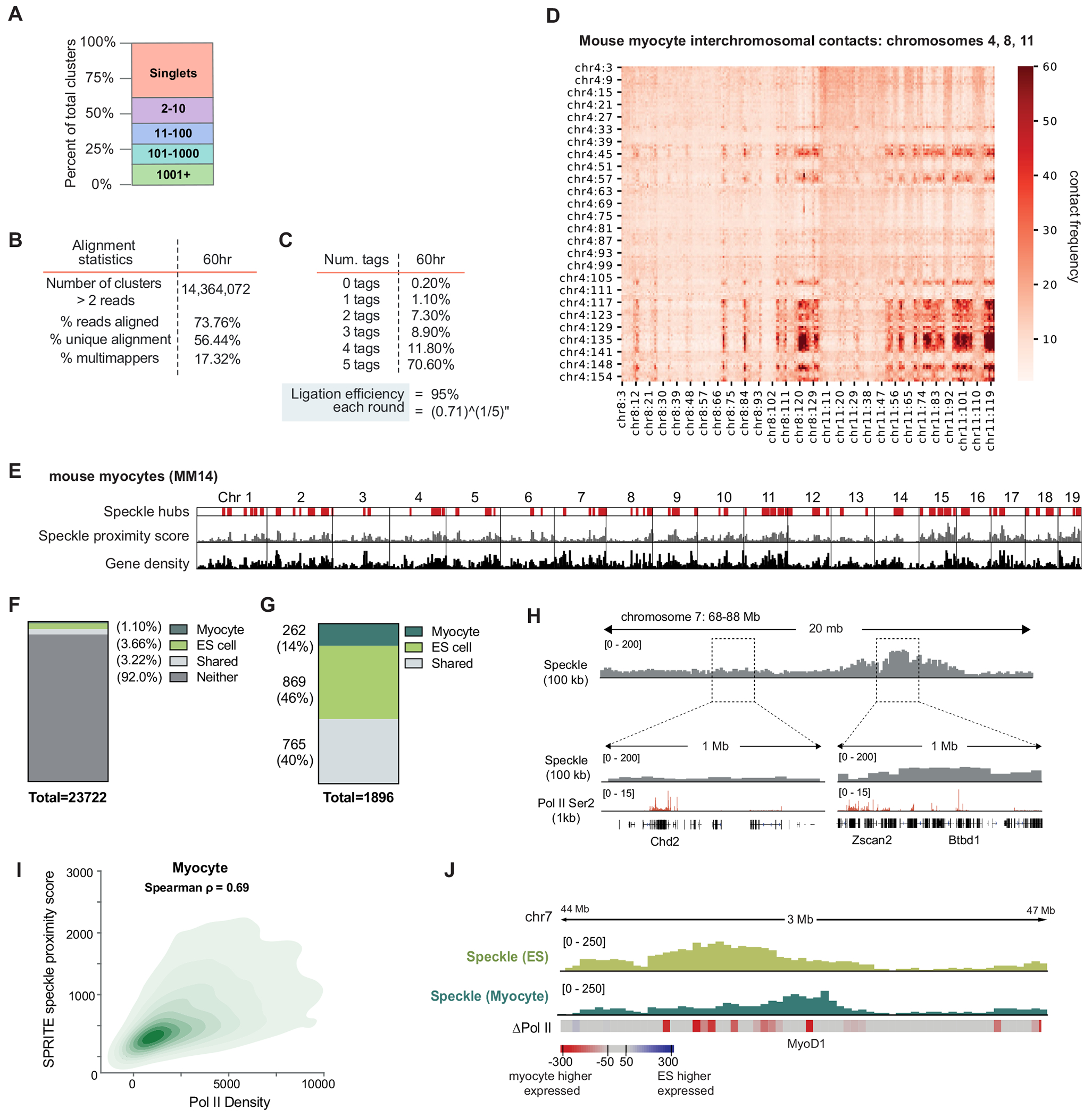
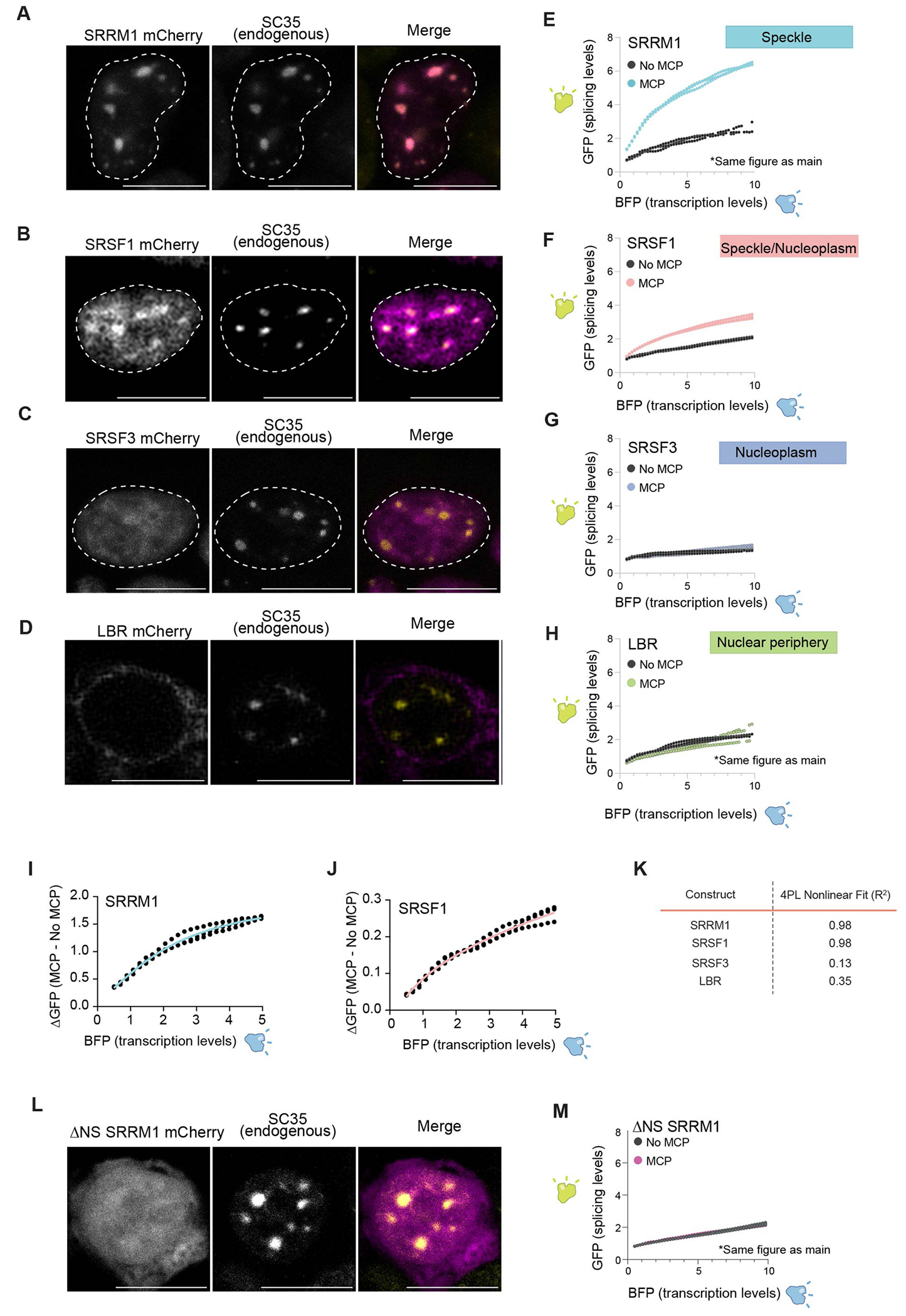
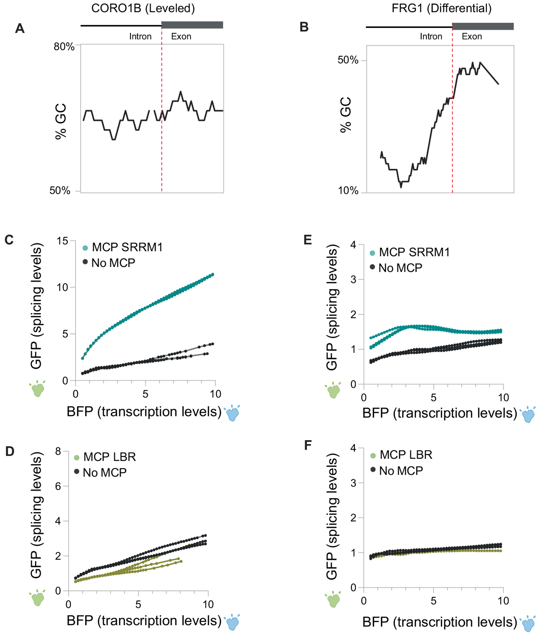
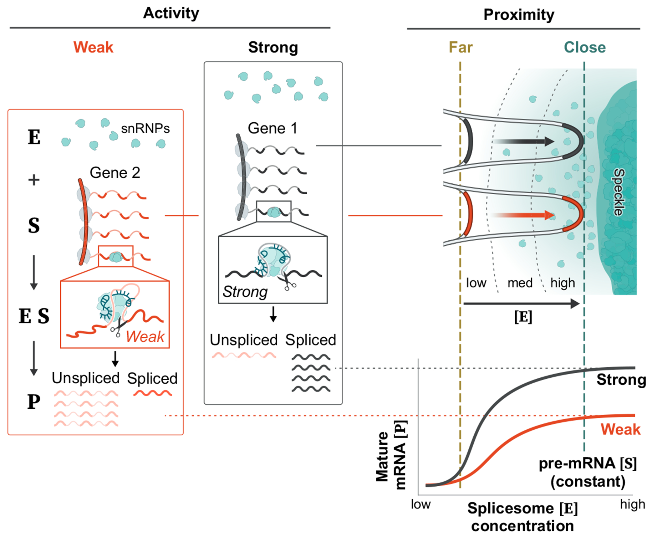
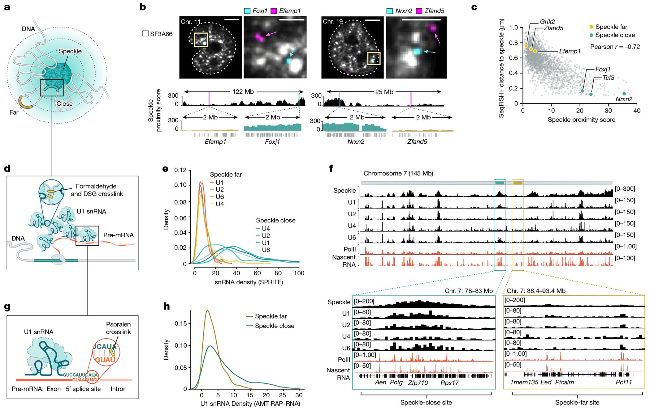
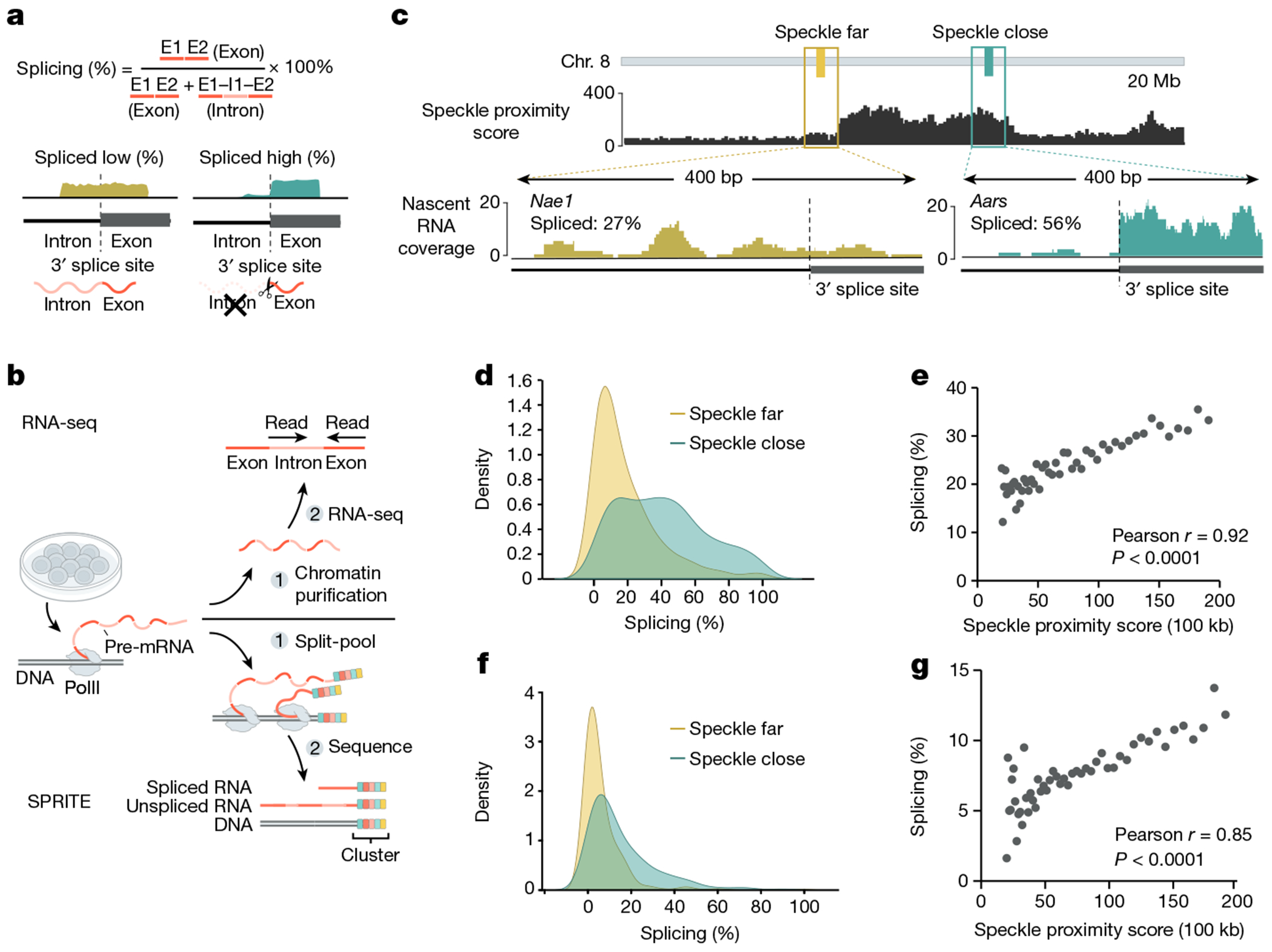
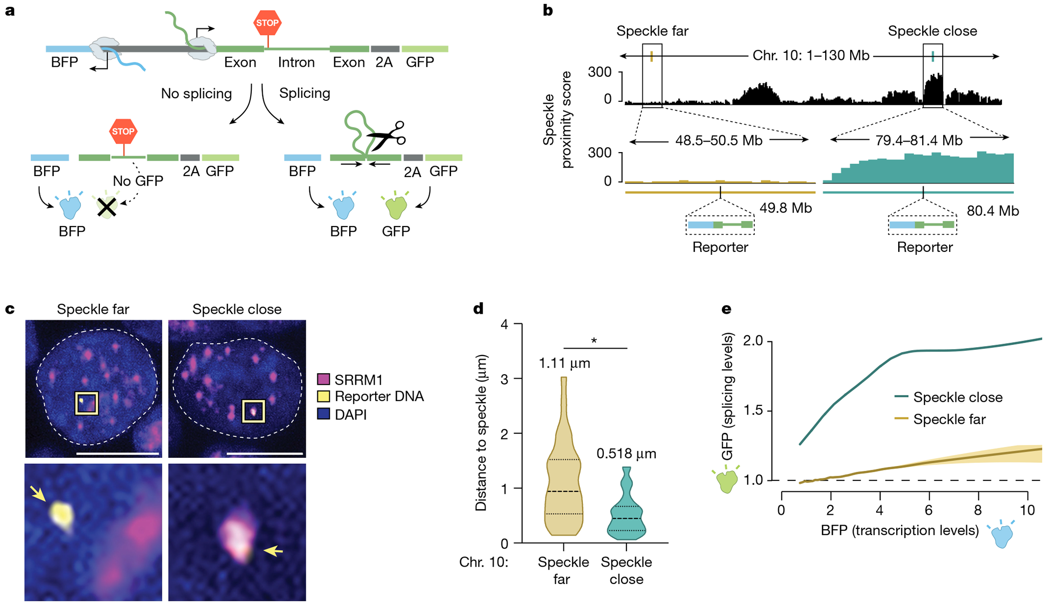
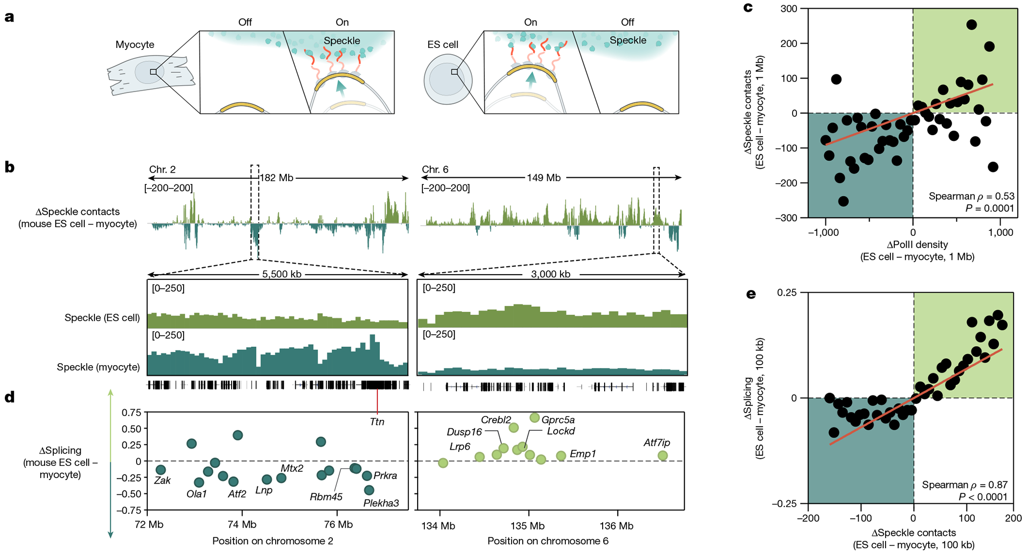
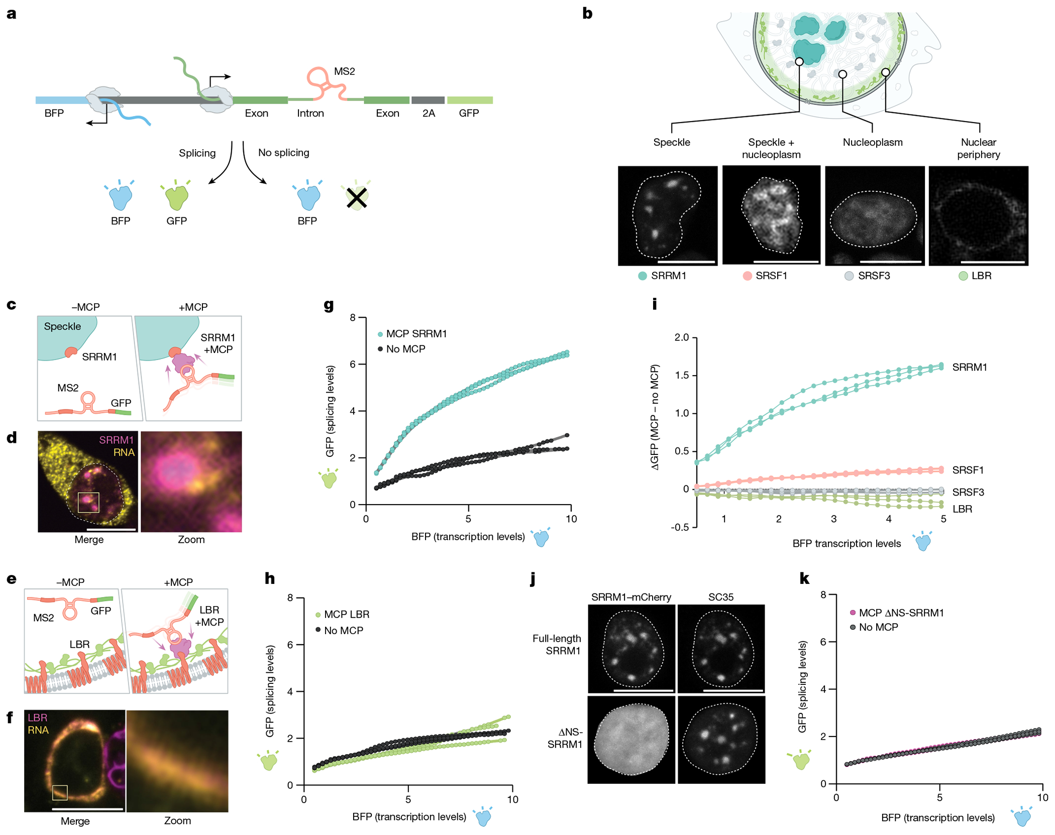
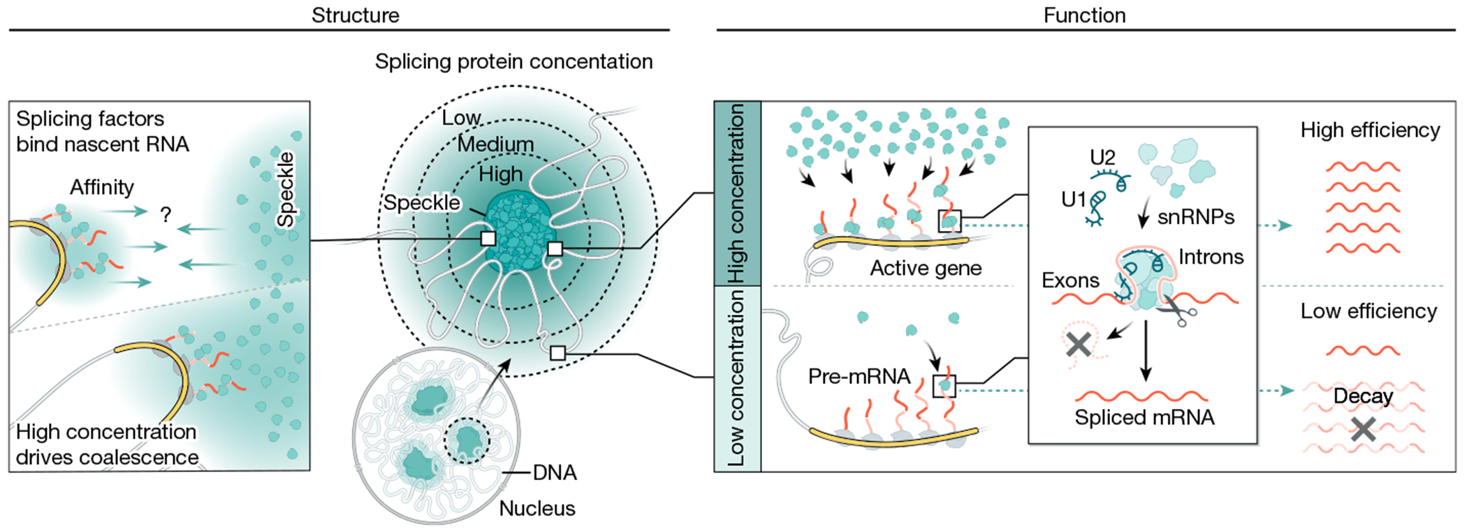
The nucleus is highly organized, such that factors involved in the transcription and processing of distinct classes of RNA are confined within specific nuclear bodies^1,2. One example is the nuclear speckle, which is defined by high concentrations of protein and noncoding RNA regulators of pre-mRNA splicing³. What functional role, if any, speckles might play in the process of mRNA splicing is unclear^4,5. Here we show that genes localized near nuclear speckles display higher spliceosome concentrations, increased spliceosome binding to their pre-mRNAs and higher co-transcriptional splicing levels than genes that are located farther from nuclear speckles. Gene organization around nuclear speckles is dynamic between cell types, and changes in speckle proximity lead to differences in splicing efficiency. Finally, directed recruitment of a pre-mRNA to nuclear speckles is sufficient to increase mRNA splicing levels. Together, our results integrate the long-standing observations of nuclear speckles with the biochemistry of mRNA splicing and demonstrate a crucial role for dynamic three-dimensional spatial organization of genomic DNA in driving spliceosome concentrations and controlling the efficiency of mRNA splicing.

Extended Data Fig. 1 |. Correlation between speckle proximity scores between SPRITE datasets and TSA-seq for SON.

A. Chromosome wide view of speckle proximity score at 1 Mb-resolution for three replicates of SPRITE datasets in mouse ES cells. Two collected in Quinodoz et al Cell 2021 and a third dataset collected for this manuscript. Speckle hub regions highlighted on chromosomes in red. Gene density track on bottom. Correlation of SPRITE experiments between: B. RD SPRITE Cell 2021 (Replicate 1) and RD SPRITE Cell 2021 (Replicate 2) (spearman r = 0.94, p < 0.0001, P value is two-tailed). C. RD SPRITE Cell 2021 (Replicate 1) and Bhat et al 2024 (spearman r = 0.90, p < 0.0001, P value is two-tailed). D. RD SPRITE Cell 2021 (Replicate 2) and Bhat et al 2024 (spearman r = 0.87, p < 0.0001, P value is two-tailed). E. Correlation of SPRITE and TSA-seq for speckle protein, SON, in H1 hESCs (spearman r = 0.75, p < 0.0001, P value is two-tailed). F. Chromosome wide view of speckle proximity score (top track) and TSA-seq (middle track, values > 0 shown) at 100-kb resolution for H1 hESCs. Gene density shown on bottom.

Extended Data Fig. 2 |. snRNA density for differently expressed genomic regions and different nascent transcription density.

A. To ensure that splicing factor difference were not due to expression differences between speckle close and speckle far genes, we divided genes up based on expression ranges: high expression (RPKM = 7.5-20), medium expression (RPKM = 2.5-7.5), low expression (RPKM = 1-2.5). The distribution of expression within these ranges were the same for speckle close and speckle far genes. The number of 100-kb regions analyzed are 8 regions each for high expression speckle close and far, 70 regions for medium expression speckle close and 28 for medium expression speckle far, and 194 for low expression speckle close and 62 for low expression speckle far. In the box plot, the center line represents the median, boxes show the interquartile range, whiskers show the range of values. B. U1 snRNA density is plotted for high (top), medium (middle), and low expression genes (bottom). C. U2 snRNA density is plotted for high (top), medium (middle), and low expression genes (bottom). D. U4 snRNA density is plotted for high (top), medium (middle), and low expression genes (bottom). E. U6 snRNA density is plotted for high (top), medium (middle), and low expression genes (bottom). (F-I): To ensure that splicing factor difference were not due to density of nascent transcription differences between speckle close and speckle far genes, we divided genes up based on transcription density ranges based on the number of nascent RNA reads from 5EU spanning each 100-kb bin. The number of 100-kb regions analyzed are 693 top 20% speckle close and 25 top 20% speckle far, 282 of 60–80% speckle close and 68 of 60–80% speckle far, 101 of 40–60% speckle close and 228 of 40–60% speckle far, 29 of 20–40% speckle close and 428 of 20–40% speckle far, and 7 of bottom 20% speckle close and 362 of bottom 20% speckle far. F. U1 snRNA density is plotted for top 20%, 60–80%, 40–60%, 20–40%, and bottom 20% of nascent transcription density. G. U2 snRNA density is plotted for top 20%, 60–80%, 40–60%, 20–40%, and bottom 20% of nascent transcription density. H. U4 snRNA density is plotted for top 20%, 60–80%, 40–60%, 20–40%, and bottom 20% of nascent transcription density. I. U6 snRNA density is plotted for top 20%, 60–80%, 40–60%, 20–40%, and bottom 20% of nascent transcription density.

Extended Data Fig. 3 |. snRNA density for junction matched genomic regions, genomic regions harboring genes of different lengths, and U1 AMT RAP-RNA enrichment for junction matched genomic regions.

A. An identical number of regions with an identical number of junctions (179 regions each for speckle close and speckle far regions)were randomly sampled to compare regions with equivalent junction density (See Methods). B. The expression levels were matched to compare the regions in A with similar mean expression per 100-kb bin. C. SPRITE speckle proximity score of filtered speckle close and speckle far regions analyzed in panel A. D. U1 snRNA density is plotted for junction and expression-controlled regions. E. U2 snRNA density is plotted for junction and expression-controlled regions. F. U4 snRNA density is plotted for junction and expression-controlled regions. G. U6 snRNA density is plotted for junction and expression-controlled regions. H. To ensure that splicing factor difference were not due to gene length differences between speckle close and speckle far genes, we divided genes up based on gene length ranges: longest genes (60^th to 80^th percentile), medium length range genes (40^th to 60^th percentile), shortest genes (bottom 20%). The distribution of length within these ranges were the same for speckle close and speckle far genes. For the regions with the longest genes, 53 speckle close and 84 speckle far 100-kb regions analyzes. For the regions with the medium length genes, 73 speckle close and 63 speckle far 100-kb regions analyzed. For the regions with the shortest genes, 178 speckle close and 102 speckle far 100-kb regions analyzed. In the box plot, the center line represents the median, boxes show the interquartile range, whiskers show the range of values. I. U1 snRNA density is plotted for longest (top), medium (middle), and shortest length genes (bottom). J. U2 snRNA density is plotted for longest (top), medium (middle), and shortest length genes (bottom). K. U4 snRNA density is plotted for longest (top), medium (middle), and shortest length genes (bottom). L. U6 snRNA density is plotted for longest (top), medium (middle), and shorted length genes (bottom). M. Density plot showing speckle proximity score (100-kb) for genomic regions enriched for U1 binding. N. U1 RAP RNA enrichment per junction (y-axis) versus number of exons per 100-kb genomic bin for speckle close and speckle far regions. Dotted lines are mean U1 enrichment values and error is SEM. Number of regions per point: n = 97, 91, 28, and 12 for speckle far regions exon number = 10, 20, 30 and 40, respectively; n = 18, 68, 70, and 47 for speckle close regions exon number = 10, 20, 30 and 40, respectively.

Extended Data Fig. 4 |. Higher splicing efficiency in speckle close regions across measurements, cell-types, and when comparing to genes of similar expression, length, and junction density to speckle far regions.

A. i. SPRITE speckle proximity score at 100-kb resolution (x axis) in mESCs and per cent spliced (from chromatin RNA-seq). 50 bins across all contact frequencies were taken and bins with speckle proximity scores between 0 and 200 are shown. Data are presented as mean values and bars represent 95% confidence interval. ii. SPRITE speckle proximity score at 100-kb resolution (x axis) in mESCs and per cent spliced (from SPRITE). 50 bins across all contact frequencies were taken and bins with speckle proximity scores between 0 and 200 are shown. Data are presented as mean values and bars represent 95% confidence interval. B. Schematic of 5EU labeling and nascent RNA sequencing pipeline. C. SPRITE speckle proximity score at 100-kb resolution (x axis) in mESCs and per cent spliced (from 5EU RNA-seq). 50 bins across all contact frequencies were taken and bins with speckle proximity scores between 0 and 200 are shown. Bars represent 95% confidence interval. Spearman r correlation = 0.95, p < 0.0001, P value is two-tailed. D. Correlation of splicing efficiency between previously published chromatin RNA-seq and newly generated 5EU RNA-seq (this paper; Spearman r correlation = 0.79, p < 0.0001), P value is two-tailed. (E-S) Splicing efficiency for speckle close and speckle far regions normalized for with genes that are: E. The top expressed genes (within 80–100% of expressed genes). 96 speckle close and 15 speckle far genes analzyed. F. Within 60–80% of expressed genes. 95 speckle close and 53 speckle far genes analyzed. G. Within 40–60% of expressed genes. 74 speckle close and 62 speckle far genes analyzed. H. Within 20–40% of expressed genes. 78 speckle close and 90 speckle far genes analyzed. I. The least expressed genes (0–20% of expressed genes). 51 speckle close and 173 speckle far genes analyzed. J. The longest genes (80–100% of genes lengths). 30 speckle close and 143 speckle far genes analyzed. K. 60–80% of gene lengths. 57 speckle close and 86 speckle far genes analyzed. L. 40–60% of gene lengths. 59 speckle close and 72 speckle far genes analyzed. M. 20–40% of gene lengths. 101 speckle close and 56 speckle far genes analyzed. N. The shortest genes (0–20% of gene lengths). 147 speckle close and 36 speckle far genes analyzed. O. 2 exons (single intron) per 100-kb region. 15 speckle close and 13 speckle far genes analyzed. P. 3–5 exons per 100-kb region. 50 speckle close and 119 speckle far genes analyzed. Q. 6–10 exons per 100-kb region. 51 speckle close and 202 speckle far genes analyzed. R. 11–15 exons per 100-kb region. 74 speckle close and 153 speckle far genes analyzed. S. 16–20 exons per 100-kb region. 95 speckle close and 78 speckle far genes analyzed. T. SPRITE speckle proximity score at 100-kb resolution (x axis) in H1-hESCs and per cent spliced within genomic bins from SPRITE (y axis) across 50 bins. Spearman r correlation = 0.70, p < 0.0001, P value is two-tailed. Median normalized speckle proximity scores are reported under each raw speckle hub contact value. Median value for H1 hESC = 7.0. U. SPRITE speckle proximity score at 100-kb resolution (x axis) in myocytes and per cent spliced (from nuclear RNA-seq) across 50 bins. Pearson r correlation = 0.64, p < 0.0001, P value is two-tailed. RD SPRITE data was not collected in myocytes for technical reasons. Median normalized speckle proximity scores are reported under each raw speckle hub contact value. Median value for mouse myocytes = 209. The range of speckle proximity scores vary between H1 hESC (1–20) and mouse myocytes (~75–400) due to the myocyte SPRITE data being sequenced more deeply.

Extended Data Fig. 5 |. Integrated reporter maintains endogenous speckle distances.

A. Representative images and zoom-ins of SRRM1 immunofluorescence combined with DNA FISH for the integrated reporter mini-gene. SRRM1 in magenta, reporter DNA in yellow and DAPI. Scale bar is 10 μm. n = 85 cells from 2 biological replicates. B. ECDF plots showing distance of DNA FISH spots of integrated location to the nearest nuclear speckle in the integrated cell lines (left) or distances computed from DNA seqFISH (right). C. Violin plots showing distance of DNA FISH spots of integrated location to the nearest nuclear speckle in the integrated cell lines (left) or distances computed from DNA seqFISH (right). Same data used as in 3C. Difference in means between speckle close and speckle far regions calculated for integrated loci and endogenous loci are represented above the distributions. D. 2D FACS plots showing GFP splicing levels as a function of BFP transcription levels between speckle close and speckle far integrated cell lines.

Extended Data Fig. 6 |. SPRITE analysis of myocyte cells and comparison to mES cells.

A. Distribution of SPRITE cluster sizes for myocyte SPRITE. The percentage of reads was calculated for different SPRITE cluster sizes (1, 2–10, 11–100, 101–1000, and over 1001 reads) and reported as the percentage of total reads. Cluster size is defined as the number of reads with the same barcode. B. Alignment statistics. C. A summary of ligation efficiency statistics to confirm tags have successfully ligated to each DNA molecule. D. Mouse myocyte interchromosomal contacts on chromosomes 4, 8, 11. E. Speckle hubs in mouse myocytes highlighted in red on chromosome track. Genome wide distribution of SPRITE speckle proximity scores (100-kb resolution). Gene density track on bottom. F. Distribution of SPRITE speckle proximity scores (100-kb resolution) for normalized mES and myocyte cell SPRITE. G. Distribution of number of genomic regions categorized as speckle hubs in myocyte, ES cells, both, or neither. H. SPRITE speckle proximity score at 100-kb resolution for a 20-Mb region on chromosome 7 in mouse myocytes. Pol II-S2P ChIP-seq density at 1-kb resolution. I. Ser2-P Pol II density (x axis) and normalized speckle proximity score (100-kb resolution) for myocytes. Spearman correlation = 0.69; p < 0.0001, P value is two-tailed. Similar to previous observations in other cellular contexts, we observed that DNA regions located close to speckles correspond to genomic regions containing high-density of RNA Pol II in differentiated myocytes. J. ES cell speckle proximity score (light green) and skeletal muscle speckle proximity score (dark green) for genomic locus near MyoD1 (expressed in myocyte). ΔPol II refers to difference in Ser2P-Pol II ChIP seq signal between mES cells and myocytes at 100-kb resolution, red is high in myocyte and blue high in ES.

Extended Data Fig. 7 |. pre-mRNA organization around nuclear speckles drives splicing efficiency.

(A-D) Whole cell imaging of each protein with SC35 immunofluorescence and overlay with nucleus outlined in white for: A. SRRM1. B. SRSF1. C. SRSF3. D. LBR. Scale bars are 10 μm. Experiment was performed three times. (E-H) GFP fluorescence (splicing levels) (y axis) versus BFP fluorescence intensity for constructs with MCP or without MCP for: E. SRRM1. F. SRSF1. G. SRSF3. H. LBR. I. Difference in GFP splicing levels between SRRM1 MCP and no MCP with a four-parameter nonlinear regression. J. Difference in GFP splicing levels between SRSF1 MCP and no MCP with a four-parameter nonlinear regression. K. Four parameter logistic nonlinear fits for SRRM1, SRSF1, SRSF3, and LBR. L. Whole cell imaging of ΔNS SRRM1 with SC35 immunofluorescence overlay. Scale bar is 10 μm. Experiment was performed three times. M. GFP fluorescence (splicing levels) (y axis) versus BFP fluorescence intensity for constructs with MCP or without MCP for ΔNS SRRM1.

Extended Data Fig. 8 |. Differential versus leveled intron architectures also display speckle dependent splicing efficiency.

A. Schematic of CORO1B (leveled) intron and mapped %GC content across intron and exon boundary. B. Schematic of FRG1 (differential) intron and mapped %GC content across intron and exon boundary. C. GFP levels (y axis) versus fluorescence intensity (levels) of BFP (x axis) (bottom) for three replicates of SRRM1+/− MCP co-transfected with CORO1B splicing reporter. D. GFP levels (y axis) versus fluorescence intensity (levels) of BFP (x axis) (bottom) for three replicates of LBR+/− MCP co-transfected with CORO1B splicing reporter. E. GFP levels (y axis) versus fluorescence intensity (levels) of BFP (x axis) (bottom) for three replicates of SRRM1+/− MCP co-transfected with FRG1 splicing reporter. F. GFP levels (y axis) versus fluorescence intensity (levels) of BFP (x axis) (bottom) for three replicates of LBR+/− MCP co-transfected with FRG1 splicing reporter.

Extended Data Fig. 9 |. Integrated model for how spliceosome activity and proximity to nuclear speckles impact kinetics of splicing.

There are two components impacting the kinetics of splicing – spliceosome concentration and spliceosome activity. (i) Proximity to nuclear speckles impacts the concentration of spliceosomes at a given pre-mRNA, such that genes that are close to speckles will have higher spliceosome concentration than genes that are far from speckles. (ii) In contrast, splice site strength is defined by the activity of the spliceosome at the splice site. In this way, spliceosomes engaged at ‘strong’ splice sites would have higher activity while ‘weak’ splice sites would have lower activity. These two components would be expected to have different effects on the kinetics of splicing. Specifically, modulating activity (splice site strength) would be expected to impact the maximum output of the reaction. Conversely, modulating concentration (speckle proximity) would be expected to impact the efficiency of each reaction.

Fig. 1 |. snRNAs preferentially bind pre-mRNAs of genes that are close to speckles.

a, Schematic of DNA regions close to (blue) or far from (yellow) nuclear speckles. b, Top, two reconstructed images of DNA seqFISH+ and immunofluorescence (SF3a66) in mouse ES cells comparing speckle-close (Foxj1 and Nrxn2) and speckle-far (Efemp1 and Zfand5) genes. Images are maximum-intensity z projected for a 1 μm section. White lines represent nuclear segmentation. Scale bars, 2.5 μm (zoom-in) or 5μm (zoom-out). Bottom, speckle proximity scores from SPRITE data for the corresponding genomic regions at 100-kb resolution. Zoom-in regions show speckle proximity scores for a specific genomic region (2 Mb) visualized by seqFISH+. n = 446 cells from two seqFISH+biological replicates from ref. . c, Genome-wide comparison of seqFISH+ distance to the periphery of a speckle (determined by microscopy) and SPRITE speckle proximity score (determined by sequencing) for 2,460 paired regions. d, Schematic of U1–DNA contacts measured by SPRITE. Formaldehyde and DSG crosslinked nucleic acids and proteins and SPRITE measure the number of molecules within each crosslinked complex. e, Density of U1, U2, U4 and U6 snRNA contacts across 100-kb genomic bins for speckle-close and speckle-far genomic regions. The distributions are quantile-normalized to have the same range as U1 to enable visualization of all snRNAs on the same scale. f, Speckle proximity scores at 100-kb resolution across chromosome 7 (top) and zoom-in views at 100-kb resolution (bottom) for a speckle hub, U1, U2, U4 and U6 snRNAs. PolII-S2P chromatin immunoprecipitation with sequencing (ChIP–seq) and nascent RNA data (10 min of 5EU) densities at 1-kb resolution. g, Schematic of direct RNA–RNA interactions by RAP-RNA. Psoralen forms direct crosslinks between RNA–RNA hybrids, and affinity purification selectively captures U1 and its directly hybridized pre-mRNAs. h, U1 density over each 5’ splice site within a pre-mRNA measured by RAP-RNA and binned within 100-kb ChIP–seq genomic bins corresponding to speckle-close and speckle-far regions. Illustrations in a, d and g created by Inna-Marie Strazhnik, Caltech.

Fig. 2 |. Co-transcriptional splicing efficiency varies based on the proximity to nuclear speckles.

a, Schematic of nascent RNA splicing efficiency calculation. Splicing efficiency of a gene is calculated by taking the ratio of exon to total pre-mRNA counts from RNA-seq (exons + introns). b, Schematic of nascent RNA-seq and SPRITE methods used to measure splicing efficiency. c, Top, SPRITE speckle proximity score for a 20-Mb region on mouse chromosome 8. Bottom, nascent RNA coverage from chromatin RNA-seq for a speckle-far (Nae1) and speckle-close (Aars) gene around a single 3’ splice site. Per cent spliced across entire gene is indicated. d, Density plot from chromatin RNA-seq of per cent spliced for genes located within speckle-close or speckle-far 100-kb genomic regions (461 speckle-close genes and 460 speckle-far genes). e, SPRITE speckle proximity score (x axis) and per cent spliced for genes from nascent RNA-seq within each bin (y axis) across 50 bins. Each point or bin contains at least 20 genes and reflects the average splicing for that bin. f, Density plot of per cent spliced within 100-kb genomic intervals from SPRITE for speckle-close and speckle-far regions (312 speckle-close and 311 speckle-far 100-kb regions). g, SPRITE speckle proximity score (x axis) and per cent spliced within genomic bins from SPRITE (y axis) across 50 bins. Each point or bin contains at least 20 regions and reflects the average splicing for that bin. Illustrations in a and b created by Inna-Marie Strazhnik, Caltech.

Fig. 3 |. Expression of a gene from a genomic locus in proximity to nuclear speckles leads to increased mRNA splicing.

a, Schematic of the bidirectional reporter assay using a fluorescence-based readout. The splicing reporter contains an exon–intron–exon minigene fused in-frame to a GFP that is translated when spliced but not when unspliced. The spliced GFP reporter is linked to a bidirectionally transcribed BFP reporter that is expressed and translated regardless of whether it is spliced. b, SPRITE speckle proximity score (100-kb bin) for the two genomic regions on mouse chromosome 10 where the reporter was integrated. c, Representative images and zoom-in images of SRRM1 immunofluorescence combined with DNA FISH for cells containing the two integrated reporters. Scale bar, 10 μm. n = 85 cells over two biological replicates. d, Violin plots of the distance of DNA FISH spots of speckle-far and speckle-close integrated loci to the nearest nuclear speckle (immunofluorescence of SRRM1) across multiple cells (n = 28 speckle-far and n = 57 speckle-close). Mean distance is displayed above each distribution. *P < 0.0001. e, GFP expression (fluorescence intensity) as a function of BFP transcription levels for speckle-close and speckle-far integrated loci. We estimated the variation of these measurements using a bootstrap procedure from ten random bootstraps generated from these data (Methods). n = 744,019 cells analysed for speckle-close and n = 158,971 cells analysed for speckle-far. P value from two-sided t-test. Illustrations in a and b created by Inna-Marie Strazhnik, Caltech.

Fig. 4 |. Differential gene positioning around speckles leads to different splicing efficiencies across cell types.

a, Schematic of the differential localization of genomic DNA relative to nuclear speckles and its dependence on PolII activity. b, Top, difference in speckle proximity score between mouse ES cells and myocytes for chromosomes 2 and 6. Bottom, 5.5-Mb and 3-Mb zoom-in regions of speckle proximity scores around the Ttn (myocyte preference) and Crebl2 (mouse ES cell preference) loci, respectively. c, Difference in PolII-S2P density (x axis) versus difference in SPRITE speckle proximity score (y axis) between ES cells and myocytes at 1-Mb resolution. n = 48 bins each containing at least 10 regions. d, Difference in splicing between mouse ES cells and myocytes for genomic regions expressed in both cell types for the same zoom-in regions as in c. Individual genes are labelled. To calculate the change in splicing efficiency between cell types, we only included genes expressed in both cell types. e, Difference in speckle proximity score (x axis) versus difference in splicing (y axis) between ES cells and myocytes at 100-kb resolution. n = 41 bins each containing at least 20 regions. P value is two-tailed (c,e). Illustration in a created by Inna-Marie Strazhnik, Caltech.

Fig. 5 |. Pre-mRNA organization around nuclear speckles drives splicing efficiency.

a, Schematic of the pre-mRNA splicing assay using a bidirectional GFP and BFP fluorescence-based readout. The MS2 stem–loop is embedded within the intron. GFP is expressed only when the reporter is spliced and was measured by FACS. b, Top, schematic of specific nuclear locations (speckle, speckle + nucleoplasm, nucleoplasm and nuclear periphery). Bottom, mCherry fluorescence of their corresponding proteins (SRRM1, SRSF1; SRSF3 and LBR). The nucleus is outlined in white. n = 3 biological replicates. c, Schematic of SRRM1 tagged with mCherry with or without a MCP tag. The MCP protein binds to the complementary MS2 stem–loop embedded within the intron of the pre-mRNA reporter. d, Single-molecule RNA FISH and zoom-in images of the localization of SRRM1 and MCP with the mCherry reporter. Nucleus is outlined in white. n = 3 biological replicates. e, Schematic of LBR tagged with mCherry with or without a MCP tag. f, Single-molecule RNA FISH and zoom-in images of the localization of LBR and MCP with the mCherry. n = 3 biological replicates. g, Fluorescence intensity of GFP (y axis) versus BFP (x axis) for three replicates of SRRM1 ± MCP. h, Fluorescence intensity of GFP (y axis) versus BFP (x axis) for three replicates of LBR ± MCP. i, Difference of GFP expression between constructs with or without MCP (y axis) versus BFP fluorescence intensity (x axis) for all constructs tested. Three replicates plotted for each sample. j, Fluorescence microscopy for mCherry±SRRM1 (top left) and mCherry ΔNS-SRRM1 (bottom left) with co-immunofluorescence for SC35 (top right and bottom right). n = 3 biological replicates. k, GFP levels (y axis) versus fluorescence intensity (levels) of BFP (x axis) (bottom) for three replicates of SRRM1 ΔNS-SRRM1 ± MCP. Scale bars, 10 μm (b,d,f,j). Illustrations in a–c and e created by Inna-Marie Strazhnik, Caltech.

Fig. 6 |. Integrated model of how gene organization around nuclear speckles affects splicing.

Model of how 3D genome organization drives mRNA splicing. Because nascent pre-mRNAs have high affinity for splicing factors and because PolII-dense regions contain the highest concentrations of nascent pre-mRNAs, these genomic regions can achieve multivalent contacts with splicing factors that are enriched within nuclear speckles. Because nuclear speckles contain the highest concentration of these factors within the nucleus, these multivalent contacts may drive coalescence (self-assembly) of these genomic DNA sites with the nuclear speckle. Genomic regions and pre-mRNAs close to nuclear speckles have higher levels of spliceosomes than regions farther away. Locally concentrating pre-mRNAs, genomic DNA and spliceosomes at speckle-proximal regions leads to increased splicing efficiency, whereas a speckle-far gene transcribed at the same level is not spliced as efficiently. Model created by Inna-Marie Strazhnik, Caltech.

References

1. Bhat P, Honson D & Guttman M Nuclear compartmentalization as a mechanism of quantitative control of gene expression. Nat. Rev. Mol. Cell Biol 22, 653–670 (2021). - PubMed
1. Dundr M & Misteli T Biogenesis of nuclear bodies. Cold Spring Harb. Perspect. Biol 10.1101/cshperspect.a000711 (2010). - DOI - PMC - PubMed
1. Spector DL & Lamond AI Nuclear speckles. Cold Spring Harb. Perspect. Biol 3, a000646 (2011). - PMC - PubMed
1. Mattaj IW Splicing in space. Nature 10.1038/372727a0 (1994). - DOI - PubMed
1. Lewis JD & Tollervey D Like attracts like: getting RNA processing together in the nucleus. Science 288, 1385–1389 (2000). - PubMed