Neurotransmitter classification from electron microscopy images at synaptic sites in Drosophila melanogaster

Abstract

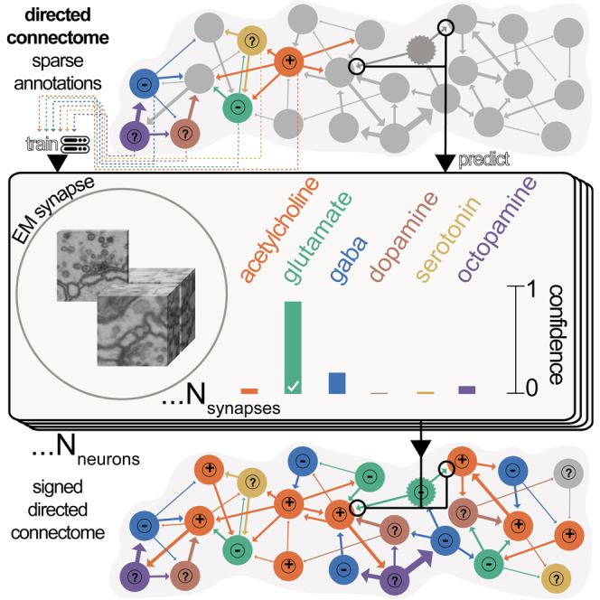
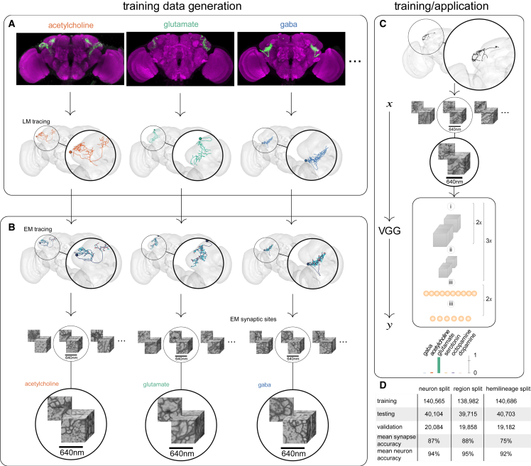
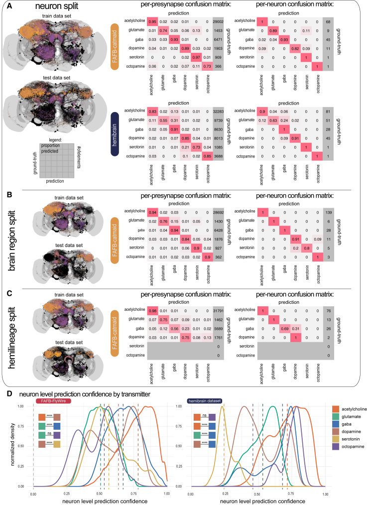
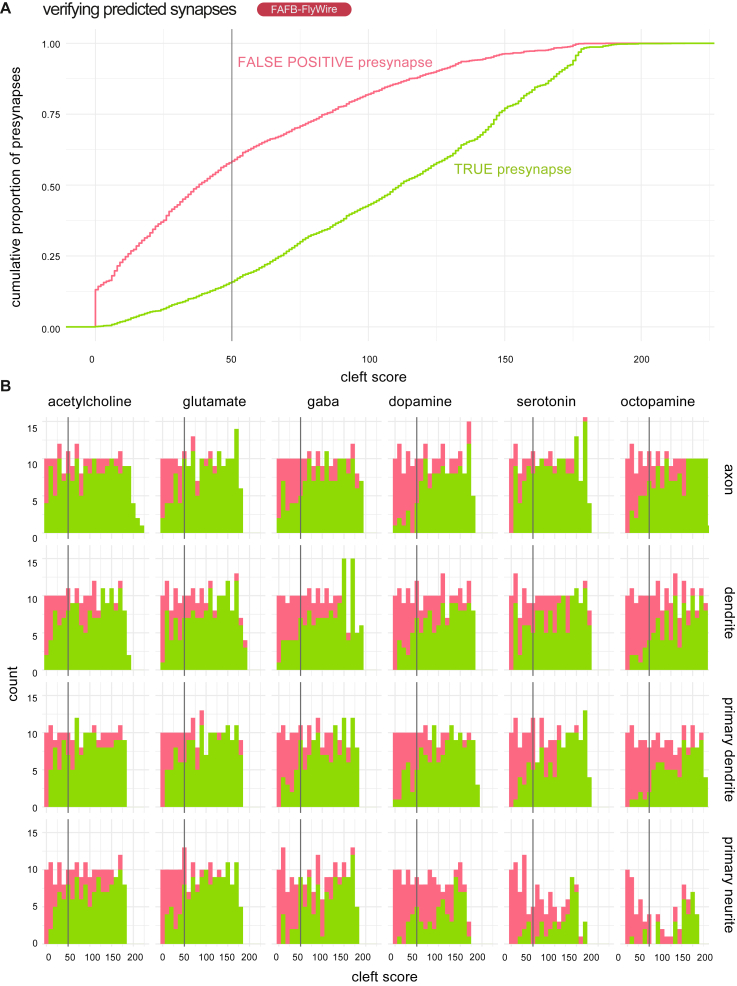
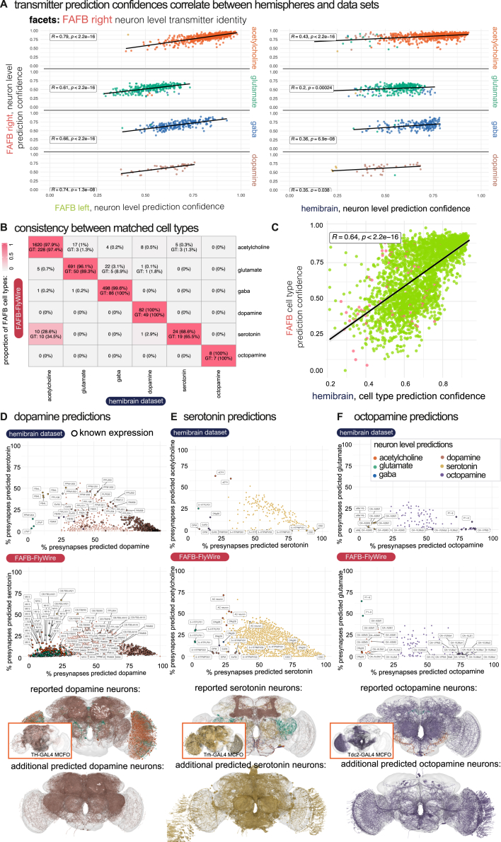
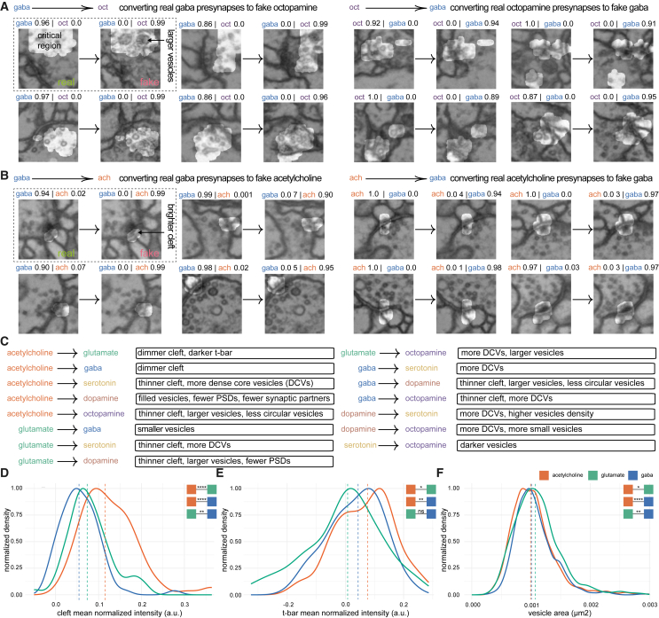
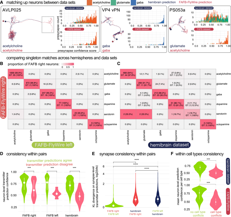
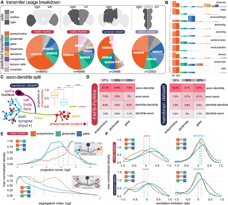
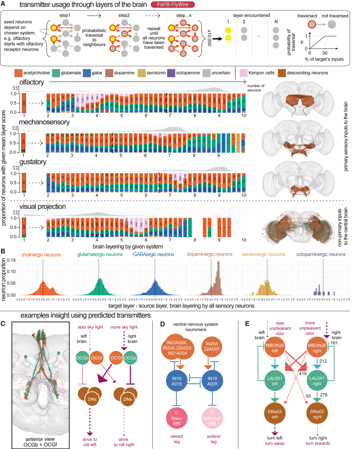
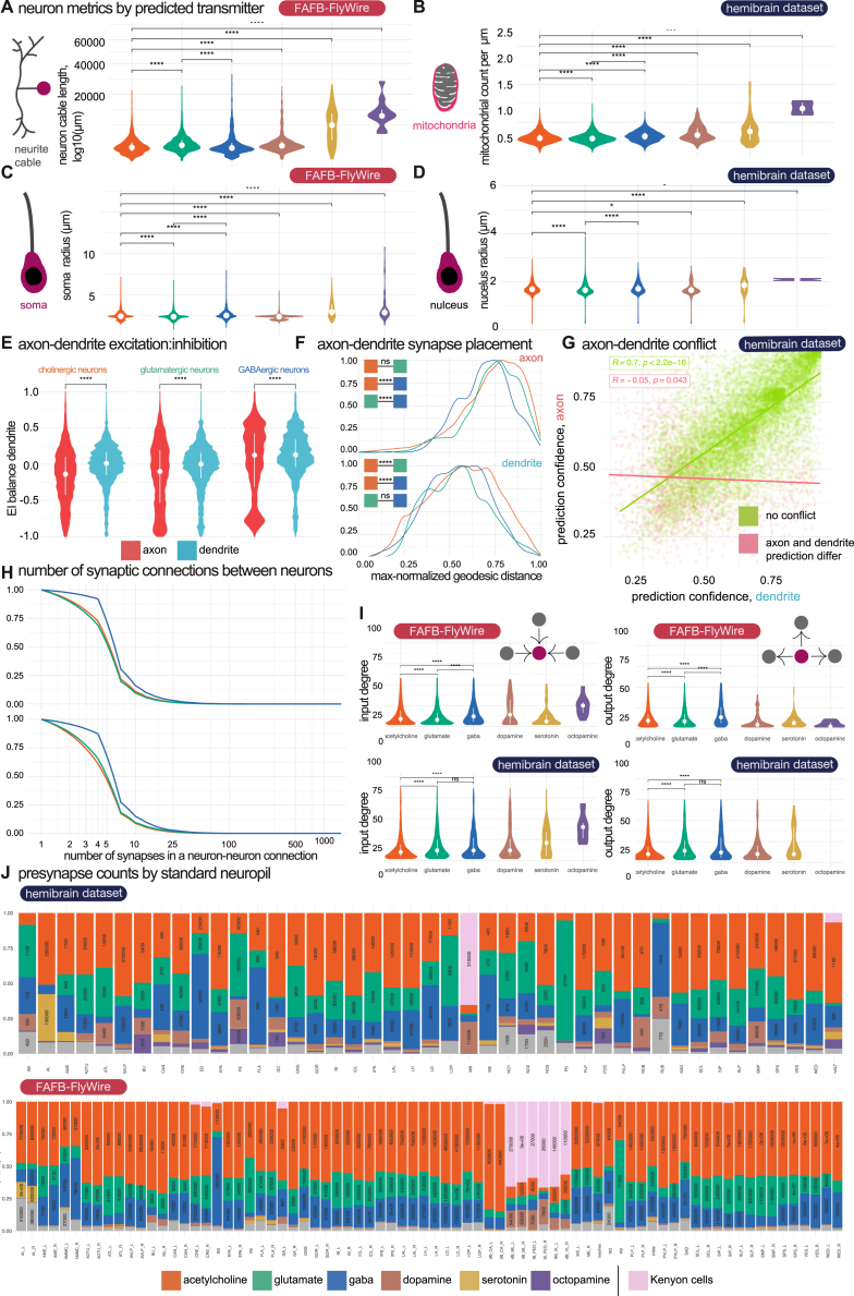
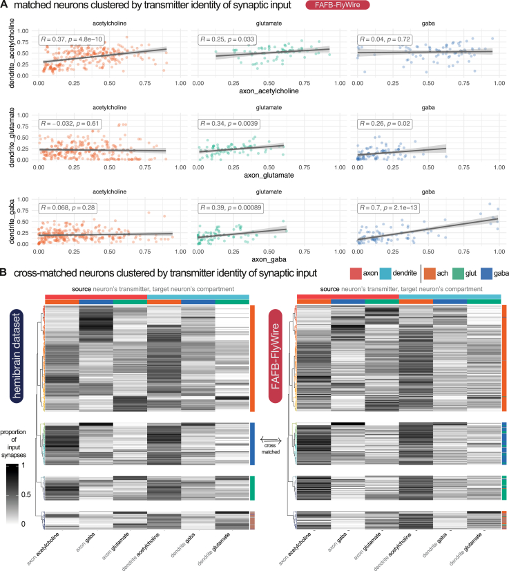
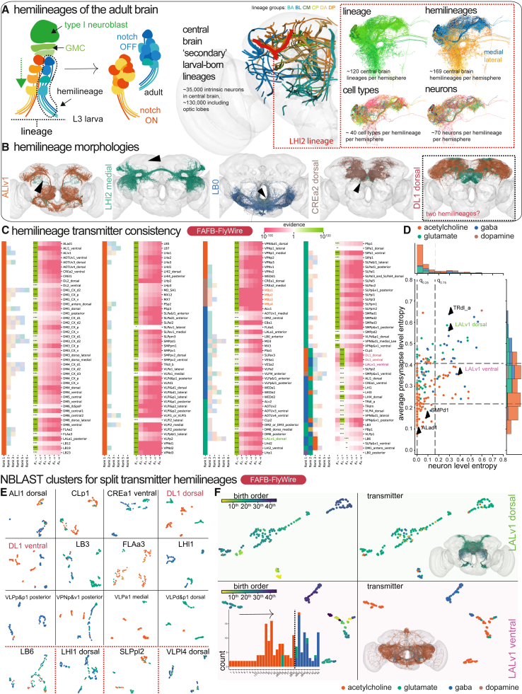
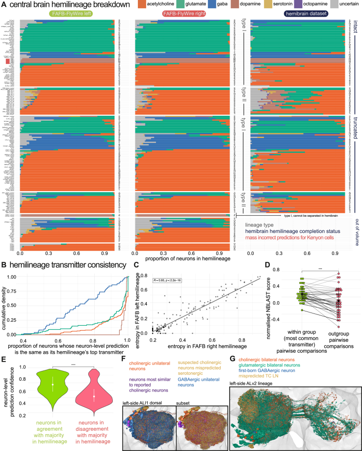
High-resolution electron microscopy of nervous systems has enabled the reconstruction of synaptic connectomes. However, we do not know the synaptic sign for each connection (i.e., whether a connection is excitatory or inhibitory), which is implied by the released transmitter. We demonstrate that artificial neural networks can predict transmitter types for presynapses from electron micrographs: a network trained to predict six transmitters (acetylcholine, glutamate, GABA, serotonin, dopamine, octopamine) achieves an accuracy of 87% for individual synapses, 94% for neurons, and 91% for known cell types across a D. melanogaster whole brain. We visualize the ultrastructural features used for prediction, discovering subtle but significant differences between transmitter phenotypes. We also analyze transmitter distributions across the brain and find that neurons that develop together largely express only one fast-acting transmitter (acetylcholine, glutamate, or GABA). We hope that our publicly available predictions act as an accelerant for neuroscientific hypothesis generation for the fly.

Keywords: neuroscience, machine learning, electron microscopy, Drosophila melanogaster, neurotransmitter, explainable AI.

Graphical abstract

Figure 1

Method overview We assembled a dataset of neurons with known transmitter expression (see STAR Methods) in two D. melanogaster brain EM datasets (FAFB and HemiBrain) and retrieved corresponding synaptic locations. (A) Typically, neurons had been genetically tagged to identify their transmitter identity and reconstruct their coarse morphology using light microscopy (Data S1). (B) Light microscopy tracings of neurons are then matched to corresponding EM reconstructions with annotated synaptic locations, yielding a dataset of EM volumes of synaptic sites with known transmitter identity. (C) We used the resulting pair (x, y) where x is a 3D EM volume of a synaptic site and y is the transmitter of that synaptic site (one of GABA, acetylcholine, glutamate, serotonin, octopamine, or dopamine) to train a 3D VGG-style deep neural network to assign a given synaptic site x to one of the six considered transmitters. We used the trained network to predict the transmitter identity of synapses from neurons with so far unknown transmitter identity. Panels i, ii, and iii denote convolution, down-sampling, and fully connected layers, respectively. (D) Overview of our results on the FAFB dataset. Shown are the number of presynapses for training, testing, and validation as well as average synapse and neuron classification accuracy on the testing set for each data split. See also Data S2.

Figure 2

The accuracy of the trained classifier on a per-presynapse and per-neuron basis (A) Left: visualization of the training (upper) and testing (lower) data (split by entire neurons) that we used for the results in this manuscript. Presynapse locations are color coded according to their z-depth; anterior-posterior shown as purple-orange, neuron skeletons in black. Right: confusion matrices for the trained classifier on the testing data, shown per presynapse and as a majority vote per neuron, on datasets FAFB and HemiBrain. We considered only those neurons with more than 30 presynapses. (B) Classification results on alternative training and testing data (split by brain regions) from FAFB. (C) Same as (B) but split by hemilineage. It was not possible to generate a fully balanced split and as a result there are no serotonin and octopamine neurons in the testing set, as indicated by the grayed-out rows. (D) The distribution of neuron-level confidence scores by transmitter, across our pool of central brain neurons in the FlyWire and HemiBrain datasets (FAFB-FlyWire, 136,927; HemiBrain, 24,666). Vertical dashed line, median value. Colored boxes with stars indicate statistical comparisons, Wilcoxon two-sample tests (n.s., not significant; ^∗p ≤ 0.05; ^∗∗∗∗p ≤ 0.00001). See also Figure S1 and Data S3 and S4.

Figure S1

Human review of auto-detected presynapses in the FAFB-FlyWire dataset, related to Figures 3 and 2 (A) Empirical cumulative density distribution curve for review of 4,306 automatically detected preynapses from the FAFB-FlyWire dataset. A presynapse comprises the synaptic machinery and vesicles on the source neuron’s side of the synaptic cleft. Detected preynapses have a “cleft score” that ranges between 0 to over 200, which indicates how discriminable the synaptic cleft at the presynaptic site is for the detection network. Our threshold of 50 is indicated by a vertical grey line. Green, determined to be a true presynapse by a human annotator; pink, determined to not be a true presynapse. (B) Rates of false presynapse detection across cleft scores, transmitter types, and compartments. We sampled ∼180 for each set of conditions. We sampled ∼10 presynapses per cleft score bin (width 10), presynaptic transmitter prediction type (columns) and neuronal compartment (rows). Histograms show the number of presynapses determined to be real (green) or not (red) by a human annotator (A.S.B). Presynapses were reviewed using the flywire interface.

Figure S2

Comparing neurons’ transmitter predictions between connectome datasets from separate animals (FAFB-FlyWire and HemiBrain) and between two hemispheres in the same dataset (FAFB-FlyWire), related to Figures 4 and 5 (A) Left. Scatterplots comparing neuron-level confidence scores in the transmitter prediction of FAFB-FlyWire-right central brain neurons, faceted by the neuron-level transmitter prediction for the FAFB-FlyWire right side homolog. Individual points colored by their FAFB-FlyWire-left or HemiBrain neuron-level transmitter prediction. Only 40 (2.5%) disagree with the FAFB-FlyWire left side prediction and 94 (7.7%) disagree HemiBrain. Right, scatterplots comparing neuron-level confidence scores in the transmitter prediction of HemiBrain dataset central brain neurons. Individual points colored by their HemiBrain side neuron-level transmitter prediction score. Only 94 (7.7%) disagree with the HemiBrain prediction. (B) A confusion matrix showing the neuronal cell type level prediction (mode of the neuron-level transmitter predictions per neuronal cell type) for neuronal cell types in the FAFB-FlyWire and HemiBrain datasets. Cells give the number of cross-matched neuronal cell types we examined, and the number of those present in the ground truth data for at least one of the two datasets. (C) A scatterplot showing the correlation between our mean prediction confidence scores for FAFB-FlyWire and HemiBrain neuronal cell types. Each point is a neuronal cell type identified in both datasets (2626). Green points mean that the transmitter prediction agrees between the two datasets and pink points indicate disagreement. Scatterplots display Pearson’s product-moment correlation, giving R, the coefficient and the associated p-value. (D) A look at dopamine predicted neurons. We show two scatterplots using data and predictions from the HemiBrain (upper) and FAFB-FlyWire (lower) datasets. The proportion of presynapses in each neuron (each point) that are predicted as dopamine (X axis) and serotonin (Y-axis). Neurons that have been predicted as dopaminergic, or known as dopaminergic from the literature (dark circles), are shown. Those neurons from the ground truth data are circled with a black ring. Upper brain plot shows neurons known to be dopaminergic (colored by their neuron-level transmitter prediction). The visual system Mi15 neurons are thought to express dopamine and acetylcholine. Lower, brain plot shows neurons strongly predicted to be dopaminergic (>50% of presynapses ‘voting’ for dopamine), excluding those in the upper plot. Many weakly predicted dopaminergic neurons belong to the central complex and mushroom body, where the density of presynapses from other neurons may have contributed to possible mis-predictions (see STAR Methods). Image inset with orange border shows light-level single neuron skeletons from MultiColor FlpOut experiments from the FlyCircuit project, from the TH-GAL4 line which labels most putative dopaminergic neurons in the fly brain. All neurons have been transformed onto the right hemisphere of the standard FlyCircuit template brain, FCWB. We have found the FlyCircuit MultiColor FlpOut data (23513 morphologies) to be unfaithful to the expected expression patterns for Cha-GAL4 (cholinergic neurons), vGlut-GAL4 (glutamatergic neurons) and Gad1-GAL4 (GABAergic neurons) and therefore of limited use in assigning transmitters, but provide the data for monoamines here to give the reader some impression of what whole brain expression patterns may look like. (E) Same as a, but for serotonin predictions. Some PPL101-6 neurons are may co-express dopamine and serotonin but are predicted as dopaminergic. Some known serotonergic neurons have low proportions of presynapses predicted as serotonergic. Flycircuit neurons from the Trh-GAL4 driver shown in inset. Trh is involved in serotonin biosynthesis. (F) Same as a, but for octopamine predictions. Flycircuit neurons from the Tdc2-GAL4 driver shown in inset, which labels putative octopaminergic and tyraminergic neurons. Most octopamine neurons have been identified in prior work. Many of our octopamine predictions (no dark circle) indicate neurons that express some other dense core vesicle transmitter in abundance, for example, PI neurons which express an insulin-like peptide. Interestingly, the putative octopaminergic aMe14b neurons (also known as OA-AL2b2 neurons) are predicted for acetylcholine. Busch et al. noted that they might not be octopaminergic, as not all neurons in cluster AL2 of NP7088 are OA-immunoreactive, and because OA-AL2b2 (HemiBrain type: aMe14b) was identified in NP7088, but not in tdc2-GAL4. OA-ASM (HemiBrain type: aMe14b) neurons also are not predicted octopaminergic, but serotonergic. On OA-ASM, Busch et al. note: “There are 8 OA-immunoreactive somata localized to the anterior superior medial protocerebrum uniquely labeled by tdc2-GAL4 (the ASM cluster). Yet they are not necessarily octopaminergic, as there are GAL4-positive neurons without OA-immunoreactivity in this cluster."

Figure 3

Classifier feature analysis using a discriminative attribution method (A) Example translations of real synapse images to fake counterfactual images. Highlights show attribution masks indicating the most important changes between the two classes. Classifier scores are shown above each image. Left, two columns show the translation of real GABA synapses into counterfactual octopamine synapses. Right, same as left but for octopamine to GABA. (B) Same as (A) but for GABA-acetylcholine. (C) Pairwise differences between transmitters, found through manual inspection of real and counterfactual images. Dense core vesicles, DCVs; postsynaptic densities, PSDs. (D) Normalized density plot showing the distribution of cleft intensity among original synapse images. Number of annotated synapses: acetylcholine 84, glutamate 61, GABA 74. (E) Same as (C) for T-bar intensities. Number of annotated synapses: acetylcholine 85, glutamate 62, GABA 75. (F) Same as (C) for vesicle sizes. Number of annotated vesicles: acetylcholine 1,729, glutamate 1,153, GABA 1,382. Vertical dashed line, median value. Colored boxes with stars indicate statistical comparisons, Wilcoxon tests. Note that the vesicle size comparison assumes that vesicle sizes from the same synapses are conditionally independent given the transmitter (n.s., not significant; ^∗p ≤ 0.05; ^∗∗p ≤ 0.001; ^∗∗∗∗p ≤ 0.00001). See also Figure S1 and Data S8.

Figure 4

Comparing neuron-level transmitter predictions between connectome datasets from separate animals and between hemispheres (A) Images of co-registered, matched neurons between the HemiBrain (navy) and the FAFB-FlyWire (red) datasets. Histograms show synapse-level transmitter prediction scores for exemplar pairs. Neurons can be matched despite missing data (left, grey dashed box). PS053a has conflicting neuron-level transmitter predictions. (B) Confusion matrix compares matched singleton FAFB-FlyWire-right and FAFB-FlyWire-left pairs’ neuron-level transmitter predictions (1,586 pairs). (C) Confusion matrix comparing matched FAFB-FlyWire-right and HemiBrain-right neuron-level transmitter predictions (1,318 pairs). Cells colored by the proportion of FAFB-FlyWire right neurons of each transmitter type (row normalized) that are matched to its homolog-columns give homolog prediction. (D) Neuron-level transmitter prediction scores between matched singletons that have (red, right) or do not have (green, left) a conflict between their neuron-level transmitter predictions, across all three hemispheres. Matches:mismatches across all comparisons for FAFB-FlyWire right: 2,650:170 FAFB-FlyWire left, 1,562:40, and HemiBrain neurons, 1,088:130. (E) Comparison of similarity scores for matches (Kullback-Leibler divergence on synapse-level transmitter prediction scores). (F) The neuron-level transmitter prediction consistency among cell types that have multiple repeats, i.e., not singletons. Green, the mean neuron-level transmitter prediction confidence for cell types where all members of the type are predicted to use the same transmitter. Red, the mean neuron-level transmitter prediction confidence for cell types where not all members of the type are predicted to use the same transmitter. Violin plots show the median value (dot) and the inter-quartile range (line, 25^th to 75^th percentiles). Data were compared using Wilcoxon two-sample tests (n.s., not significant; ^∗∗∗p ≤ 0.0001; ^∗∗∗∗p ≤ 0.00001. See also Figure S2 and Data S7.

Figure 5

Breakdown of transmitter use across the D. melanogaster nervous system (A) Our neuron-level transmitter predictions across the female optic lobes and central brain and a male ventral nerve cord (see STAR Methods). (B) Bar plots for the numbers of neurons predicted for different transmitter usages in each super class in the FAFB-FlyWire dataset. (C) Schematic of a neuron broken into its neuronal compartments. Inset, the proportion of presynapses in each of the four compartment types. (D) Synaptic budget across different connection types in FAFB-FlyWire (left) and HemiBrain (right). Heatmaps show the proportion of synaptic contacts from neurons of different predicted transmitter types (columns) used in different inter-compartmental connection types (rows). FAFB-FlyWire, 9,123; hemibrain, 10,122 neurons. (E) Scaled density plots showing neuronal polarity by neuron-level transmitter prediction. Upper, distribution of projection scores, which is the distance in Euclidean space between the dendritic an axonic midpoint. Lower, segregation index: the higher the score, the more polarized the neuron. (F) Scaled density plots showing the distribution of excitation-inhibition balance (proportion of excitatory, acetylcholine, input minus the proportion of inhibitory input; GABA, glutamate) across neuron-level transmitter predictions and compartments. Vertical dashed line, median value. Colored boxes with stars indicate statistical comparisons, Wilcoxon two-sample tests (n.s., not significant; ^∗p ≤ 0.05; ^∗∗∗p ≤ 0.0001; ^∗∗∗∗p ≤ 0.00001). See also Figures S2 and S3 and Data S3 and S4.

Figure 6

Transmitter usage through sensory layers and specific circuits (A) Schematic depicts the probabilistic graph traversal model used to “layer” different sensory systems, adapted from Schlegel et al., underlying data from Dorkenwald et al. Starting from first-order central brain input neurons, we recorded the mean step (“layer”) at which each subsequent FAFB-FlyWire neuron is encountered by the simulation. Bar charts show transmitter input across distinguishable sensory systems. Bars normalized and binned by target neurons’ layer score (width 0.2); text reports neuron count. Kenyon cells are shown in pink and descending neurons, i.e., the last captured point of the sensory-motor transform in the brain, in brown so that the reader can compare layer progression between systems. Vertical line shows the mean descending neuron layer. Olfactory sensory neurons mispredicted for serotonin are corrected to acetylcholine. “Uncertain” neurons (see STAR Methods) were removed from this analysis. (B) Feedforward and feedback connectivity across sensory systems by neuron-level transmitter prediction. For each unitary neuron-neuron connection (greater than 100) between a source and target neuron, we calculated a target-source layer difference: the layer value for the target neuron minus the layer value of the source neuron. Y axis gives the proportion of unitary connections in each bin (width 0.1). (C) A potential circuit for righting the fly’s body axis relative to celestial cues. Purple arrow weight indicates activity level. (D) A potential circuit for differential leg extension/retraction control. (E) A potential circuit for steering away from unpleasant odors. Numbers give synaptic counts from HemiBrain. See also Figure S4.

Figure S3

Comparing neuron features across transmitter classes, related to Figure 5 (A) Cable length by neuron-level transmitter prediction. (B) Mitochondria density by neuron-level transmitter predictions. Violin plots show the number of automatically detected mitochondia per micron cubed. Volume measures per neuron originate from the HemiBrain’s automatically reconstructed 3D neuron volumes. A mitochondria detection is currently only available in the HemiBrain dataset. The mean number of mitochondria per neuron is 245, s.d. 275. (C) Soma, i.e., neuronal cell body, and (D) nucleus size by neuron-level transmitter predictions. The HemiBrain dataset provides a soma segmentation (left), and the FAFB-FlyWire dataset provides a nucleus segmentation (right)^,. (E) Violin plots of excitation:inhibition balance by neuron-level transmitter prediction and compartment. (F) Correlation between compartment-level transmitter prediction score for axons and dendrites. Each point is a separate neuron in the HemiBrain dataset, n = 10,122. 11.0% disagree on the compartment-level transmitter prediction (red). The scatterplot displays Pearson’s product-moment correlation, giving R, the coefficient and the associated p-value. (G) Scaled density plot showing the density of input connections onto all FAFB-FlyWire and HemiBrain neurons (facets) at different synaptic weights (X axis, log2). (H) Scaled density plots showing the max-normalised geodesic distance (the distance along a neuron’s arbour) from input synapses (colored by the source neuron’s neuron-level transmitter prediction) to the target neurons’ cell body. (I) Differences in the number of outgoing and incoming connections by neuron-level transmitter prediction. The input and output degree for a neuron is the number of unitary connections it has incoming and outgoing, respectively (the number of synaptic pairs, regardless of synaptic weight). All source-target connections with a synaptic count $\ge$ 10 included. Left, boxplots show the distribution of input degrees by the target neurons’ neuron-level transmitter prediction. Right, output degrees by the source neurons’ neuron-level transmitter prediction. A subset of total central brain neurons that were skeletonized (see STAR Methods) were used for this analysis (FAFB-FlyWire: 88,115, HemiBrain: 11,277). (J) Breakdown of neuron-level transmitter predictions by brain region in HemiBrain. Plot shows the proportion of synapses in each HemiBrain neuropil that belong to a neuron of a given neuron-level transmitter prediction (colors). A total of $\sim$ 4,000,000 were assigned a neuropil and neuron-level transmitter prediction, which helps buffer erroneous synapse-level transmitter predictions. Number labels give the total number of synapses in each group. Not all the standard neuropils are shown because the HemiBrain only comprises $\sim$ 1/3 of the central brain. Total number of neuronal reconstructions (see STAR Methods) by dataset: FAFB-FlyWire: 136,927, HemiBrain: 24,666. (J) Breakdown of neuron-level transmitter predictions by brain region in FAFB-FlyWire. Neuropils: AB, asymmetric body, AL, antennal lobe, AME, accessory medulla, AOTU, anterior optic tubercle, ATL, antler, AVLP, anterior ventrolaterla protocerebrum (incomplete in in HemiBrain), BU, bulb, CAN, cantle, CRE, crepine, EB, ellipsoid body, EPA, epaulette, FB, fan-shaped body, FLA, flange, GC, great commissure (incomplete in HemiBrain), GNG, gnathal ganglion (incomplete in HemiBrain), GOR, gorget, IB, inframedial bridge, ICL, inferior clamp, IPS, inferior posterior slope, LAL, lateral accessory lobe, LH, lateral horn, LO, lobula (incomplete in HemiBrain), LOP, lobula plate (incomplete in HemiBrain), ME, medulla (incomplete in HemiBrain), NO1, nodulus compartment 1, NO2, nodulus compartment 2, NO3, nodulus compartment 3, PB, protocerebral bridge, PLP, posterior lateral protocerebrum, POC, posterior optic commissure, PVLP, posterior ventrolateral protocerebrum (incomplete), ROB, round body, RUB, rubus, SAD, saddle, SCL, superior clamp, SIP, superior intermediate protocerebrum, SLP, superior lateral protocerebrum, SMP, superior medial protocerebrum, SPS, superior posterior slope, VES, vest, WED, wedge. Violin plots show the median value (dot) and the inter-quartile range (line, 25^th to 75^th percentiles). Significance values: ns: p > 0.05; ^∗: p ≤0.05; ^∗∗: p ≤ 0.01; ^∗∗∗: p ≤0.001; ^∗∗∗∗: p ≤ 0.0001.

Figure S4

Diversity in targeting by transmitter class and compartment, related to Figure 6 (A) Correlations between opposing input transmitter types by compartment. Plots faceted by the source (upstream) neurons’ neuron-level transmitter prediction (axis values). Colored by the target (downstream) neurons’ neuron-level transmitter prediction. The X axis shows the proportion of a neuron’s input accounted for by the input type on the axis label. Each dot is one neuron. For calculating the R² and p-values, neurons for which a proportion on either the X or Y axis fell below 0.1 or above 0.9 were excluded, to remove outlier cases with a very strong input preference. (B) Equivalent 451 neuronal cell types from the FAFB-FlyWire and HemiBrain datasets clustered by input type. Only neurons for which at least 50% of inputs came from well-reconstructed and predicted neurons in our 88,115 FAFB-FlyWire neurons or 11,277 HemiBrain neurons were used. For each source neuron to target neuron connection, we used the identity (neuron-level transmitter prediction), location (neuronal compartment) and normalized connection weight (number of synaptic contacts made on that compartment / total number of synaptic inputs to the target neuron). We calculated cell type averages, and separated target cell types by their transmitter prediction and then clustered within each grouping. Heatmaps show the proportion of synaptic input onto the axon (upper horizontal color bar, red) and dendrite (blue), separated by the neuron-level transmitter prediction for each input (lower horizontal color bar). Each row is a separate neuronal cell type (see Figure S4C for names). Cell types are grouped by a hierarchical clustering within their neuron-level transmitter prediction class (vertical color bar: acetylcholine, glutamate or GABA) employing Ward’s clustering criterion. This clustering was performed in the HemiBrain dataset and applied to the FAFB-FlyWire dataset. Dendrogram (left) colors show a split into 30 groups. The same dendrogam is used in both heatmaps. Cosine similarity, z = 0.892, p-value < 0.0001, 100,000 row shuffles. A subset of total central brain neurons that had been skeletonized (see STAR Methods) were used for these analysis (FAFB-FlyWire: 88,115, HemiBrain: 11,277).

Figure 7

Transmitter usage across all hemilineages in the central fly brain (A) Left, the progression of a type I neuroblast from third-instar larva (L3) into the adult ganglion mother cell (GMC). Right, a breakdown of a single secondary lineage, “LHl2” into its constituent hemilineages (see STAR Methods). (B) Example of homologous FAFB-FlyWire hemilineages on both sides of the brain, colored by neuron-level transmitter prediction. Black arrows point to one stray member of each hemilineage with a different neuron-level transmitter prediction, which is likely a first-born neuron with distinct morphology^, (Data S5). The dashed box indicates a hemilineage with potential split transmitter expression. (C) Bayes factor analysis of hemilineage consistency. For each hemilineage (row), the right set of columns corresponds to the likelihood ratio of the hemilineage expressing that number of transmitters versus the likelihood of any other number ($\lambda =16;{\tilde{c}}_{\exp }=0.67$). Evidence strength: substantial ^∗K ⩾ 10^1/2; good ^∗∗K ⩾ 10¹; strong ^∗∗∗K ⩾ 10^3/2; decisive ^∗∗∗∗K ⩾ 10². The left set of columns indicates the frequency ranked transmitter predictions within the hemilineage, with ranks greater than the maximum likely number of transmitters shaded lighter. “LB0 posterior” did not have substantial evidence for any particular number of transmitters. (D) Neuron level entropy (H(N_h)) versus average synapse level entropy (H(S_h)) for all predicted hemilineages with more than 10 neurons and more than 30 presynapses per neuron. Dashed lines indicate 25% and 75% percentiles: q₂₅(H(N_h)) = 0.00, q₂₅(H(S_h)) = 0.22, q₇₅(H(N_h)) = 0.17, and q₇₅(H(S_h)) = 0.41.$\text{Type}\text{equation}\text{here.}$ (E) NBLAST UMAP plots of selected hemilineages that exhibit some degree of predicted split transmitter usage. UMAPs are based on NBLAST morphological similarity scores between all possible pairs of neurons in each hemilineage. Points represent neurons, colored by neuron-level transmitter prediction. Black solid lines bound examples with a morphology-transmitter split, red dashed lines bound examples with no such clear divide. Red text label examples for which data annotation issues may explain split usage. (F) “LALv1” has two hemilineages: dorsal (developmentally defined by Notch-ON) and ventral (Notch-OFF). NBLAST UMAPs for the two “LALv1” hemilineages (rows): dorsal (developmentally defined by Notch-ON) and ventral (Notch-OFF), colored by birth order (left) and neuron-level transmitter prediction (right). Bottom left, histogram of neuron-level transmitter prediction by birth order. See also Figure S5 and Data S6.

Figure S5

The distribution of neuron-level transmitter predictions within secondary hemilineages, related to Figure 7 (A) Consistency of neuron-level transmitter predictions within selected hemilineages in the central adult D. melanogaster brain. Bar plots show the proportion of neurons in each hemilineage predicted to express each of our six transmitters. Data is shown for neurons of the left (left) and right (middle) hemispheres of the FAFB-FlyWire dataset, as well as both hemispheres of the HemiBrain dataset (right). Note that the HemiBrain dataset is only a partial brain, many brain neurons have large missing portions or do not exist in this dataset. Hemilineage names are given on the left of the bar plots, and the numbers of neurons per hemilineage are on the right. The red bar highlights lineages of cholinergic Kenyon cells, MBp1-4, which are mispredicted dopaminergic. The plot is faceted first by presence in the HemiBrain dataset (intact, truncated, missing), then by lineage type (Type I and Type II). (B) Empirical cumulative density plot shows how consistent a transmitter within each hemilineage is predicted to be. The Y axis gives the proportion of hemilineages, and the X axis gives the proportion of neurons in those hemilineages that “voted" for the top transmitter (color groups). (C) How the Shannon entropy (base 6) in the neuron-level transmitter predictions for each hemilineage correlate, between the hemilineage copy on the right (X axis) and left (Y-axis) hemispheres of the FAFB-FlyWire dataset. (D) Dot plot shows the mean normalized pairwise NBLAST scores between neurons expressing the majority transmitter within a hemilineage (for each green dot, each member of pair expresses the main transmitter) and between these neurons and those expressing other transmitters (pink, at least 10 neurons expresses the other transmitter). Dots represent means taken per hemilineage (183). (E) Violin plot shows the distribution of neuron-level transmitter prediction confidences for neurons that are in agreement with their hemilineage’s transmitter use (green, strictly obey Lacin’s law) and those that do not (pink, strictly obey Lacin’s law). (F) Majority unilateral, left-side antennal lobe local neurons of ‘ALlv1 dorsal’. Neurons colored by their neuron-level transmitter prediction except for a minority of predicted serotonergic neurons with the most ventral cel bodies, given in purple. These are the most similar to described Krasavietz positive cholinergic local neurons.^, The upper plot shows neurons predicted to transmit acetylcholine with neurons likely mispredicted to transmit serotonin; they have similar primary neurite and soma positions. We suspect they all should be predicted for acetylcholine. Lower, GABAergic predicted neurons have been added in. (G) Majority bilateral, left-side antennal lobe local neurons of ‘ALlv2’. Neuron meshes colored by neuron-level transmitter prediction. Data were compared using Wilcoxon two-sample tests. Significance values: ns: p > 0.05; ^∗: p ≤0.05; ^∗∗: p ≤ 0.01; ^∗∗∗: p ≤0.001; ^∗∗∗∗: p ≤ 0.0001.

References

1. Cook S.J., Jarrell T.A., Brittin C.A., Wang Y., Bloniarz A.E., Yakovlev M.A., Nguyen K.C.Q., Tang L.T.-H., Bayer E.A., Duerr J.S., et al. Whole-animal connectomes of both caenorhabditis elegans sexes. Nature. 2019;571:63–71. - PMC - PubMed
1. Ohyama T., Schneider-Mizell C.M., Fetter R.D., Aleman J.V., Franconville R., Rivera-Alba M., Mensh B.D., Branson K.M., Simpson J.H., Truman J.W., et al. A multilevel multimodal circuit enhances action selection in drosophila. Nature. 2015;520:633–639. - PubMed
1. Phelps J.S., Hildebrand D.G.C., Graham B.J., Kuan A.T., Thomas L.A., Nguyen T.M., Buhmann J., Azevedo A.W., Sustar A., Agrawal S., et al. Reconstruction of motor control circuits in adult drosophila using automated transmission electron microscopy. Cell. 2021;184:759–774.e18. - PMC - PubMed
1. Ryan K., Lu Z., Meinertzhagen I.A. The cns connectome of a tadpole larva of ciona intestinalis (l.) highlights sidedness in the brain of a chordate sibling. Elife. 2016;5 - PMC - PubMed
1. Takemura S.-Y., Hayworth K.J., Huang G.B., Januszewski M., Lu Z., Marin E.C., Preibisch S., Shan Xu C., Bogovic J., Champion A.S., et al. A connectome of the male drosophila ventral nerve cord. bioRxiv. 2023 doi: 10.1101/2023.06.05.543757. Preprint at. - DOI
Publication types
Substances
LinkOut - more resources