Lense-Thirring precession after a supermassive black hole disrupts a star

Abstract

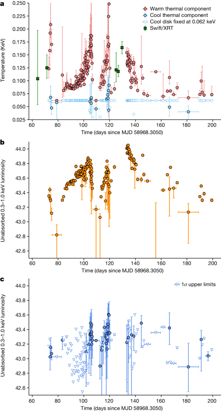
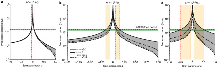
An accretion disk formed around a supermassive black hole after it disrupts a star is expected to be initially misaligned with respect to the equatorial plane of the black hole. This misalignment induces relativistic torques (the Lense-Thirring effect) on the disk, causing the disk to precess at early times, whereas at late times the disk aligns with the black hole and precession terminates^1,2. Here we report, using high-cadence X-ray monitoring observations of a tidal disruption event (TDE), the discovery of strong, quasi-periodic X-ray flux and temperature modulations. These X-ray modulations are separated by roughly 15 days and persist for about 130 days during the early phase of the TDE. Lense-Thirring precession of the accretion flow can produce this X-ray variability, but other physical mechanisms, such as the radiation-pressure instability^3,4, cannot be ruled out. Assuming typical TDE parameters, that is, a solar-like star with the resulting disk extending at most to the so-called circularization radius, and that the disk precesses as a rigid body, we constrain the disrupting dimensionless spin parameter of the black hole to be 0.05 ≲ ∣a∣ ≲ 0.5.

Fig. 1. Multi-wavelength evolution of AT2020ocn.

a, X-ray luminosity (0.3–1.0 keV) versus time since optical discovery. Gaps in NICER monitoring are filled by Swift data. The dashed and vertical lines are separated by 15 days to guide the eye. Archival Swift X-ray (0.3–1.0 keV) 3σ upper limits from before MJD 58274 is 3 × 10⁻¹⁴ erg s⁻¹ cm⁻² (4 × 10⁴¹ erg s⁻¹). The first X-ray or XRT data point is a non-detection with a 3σ upper limit of 1.7 × 10⁻¹³ erg s⁻¹ cm⁻². b, Optical and UV evolution of AT2020ocn. All values are host-subtracted. All the other error bars represent 1σ uncertainties. See ‘Data availability’ section below to access the data.

Fig. 2. LSP of the observed 0.3–1.0 keV NICER light curve.

a, The blue dashed histogram represents the unbinned LSP, whereas the red data points are the binned LSP excluding the peaks near 15 days and 2 × 15 days. The solid blue and orange curves are the best-fit bending power-law + constant and power-law + constant models, respectively, used to characterize the noise continuum. b, Unbinned periodogram (same as a but the y-axis is shown on linear scale without overplotting the continuum for clarity).

Fig. 3. X-ray spectral evolution of AT2020ocn.

a, Temperature evolution of the warm and the cool X-ray thermal components. When the cool component was not statistically required by the data, we froze its temperature to 0.062 keV and computed the 1σ upper limit on the flux of the cool component. b,c, Logarithm of luminosity of the warm component (b) and the cool component (c). All error bars represent 90% uncertainties.

Fig. 4. Spin constraints on SMBH of AT2020ocn based on the rigid body Lense–Thirring precession model.

a–c, The precession period–spin relations for the upper limit (a), best fit (b) and the lower limit (c) on the SMBH mass inferred from the M–σ_* relation (see section ‘Black hole mass from the stellar velocity dispersion of the host galaxy’). For these calculations, we assumed standard TDE parameters, that is, a solar-like star with the resulting disk extending out to tidal radius. The grey-shaded area captures the uncertainty arising from various disk–density profiles. The green dashed horizontal line represents the rest-frame period of AT2020ocn (15.9 days) and the green band reflects the uncertainty in the rest-frame period (${15.9}_{-2.2}^{+1.1}\mathrm{days}$). For a given SMBH mass, the possible spin values are shown by the orange-shaded area. The overall spin constraint for the SMBH of AT2020ocn across all masses is 0.05 ≲ ∣a∣ ≲ 0.5 (see Extended Data Table 1 for specific values).

Extended Data Fig. 1. SDSS host spectrum of AT2020ocn (black).

Overlaid in orange is the best fit MILES model template obtained through pPXF fitting, broadened to a velocity dispersion of 82 ± 4 km s⁻¹. No narrow emission lines are evident in the spectrum.

Extended Data Fig. 2. Swift/XRT 0.3-1.0 keV image of NICER’s FoV.

The yellow circle with a radius of 47″ and is centered on AT2020ocn’s optical coordinates of 13:53:53.803, +53:59:49.57 (J2000.0 epoch). The outer cyan circle shows NICER/XTI’s approximate field of view of 3.1′ radius. There are no contaminating sources within NICER’s field of view. The north and east arrows are each 100″ long. The colorbar shows the number of X-ray counts.

Extended Data Fig. 3. White noise tests for the distribution of noise powers in the observed Lomb Scargle periodogram (LSP) using power values that correspond to timescales slower than 3 days and excluding bins near 15, 2 × 15 and 4 × 15 days.

(a) Comparison of the cumulative distribution functions (CDFs) of the observed noise powers and the expected exponential distribution. The CDF of the observed LSP of the observed light curve is represented by the orange histogram, while the solid black line shows the CDF of white noise powers, which follows an exponential distribution. (b) Comparison of the probability density functions of the observed noise powers and the expected exponential distribution. The solid black line is the PDF of white noise distribution, whereas the shaded orange histogram represents the PDF of the observed noise powers in the LSP of the observed light curve. (c) Distribution of the Kolmogorov-Smirnov test statistic derived from simulations. (d) Distribution of the Anderson-Darling test statistic using simulations. In both (c) and (d), the solid red and the dashed black lines represent the median of the distribution and the observed value, respectively and the shaded blue regions indicate the ± 1σ values of their respective distributions. The null hypothesis that the noise powers are exponentially distributed, i.e., consistent with white noise, cannot be rejected.

Extended Data Fig. 4. Check for powerlaw index bias due to uneven sampling.

The distribution represents the powerlaw index values of the simulated LSPs with an input index of 1.0.

Extended Data Fig. 5. Estimates of the global false alarm probability (FAP) of finding a broad peak in the simulated LSPs.

Each panel is for a different underlying noise continuum: (a) white noise, (b) powerlaw red noise with best-fit powerlaw index, α_best−fit, and normalization, Norm_best−fit, (c) powerlaw red noise with best-fit powerlaw index + 1σ and its corresponding normalization, (d) powerlaw red noise best-fit normalization + 1σ and its corresponding powerlaw index, (e) bending powerlaw red noise with best-fit parameters, and (f) bending powerlaw red noise with best-fit normalization + 1σ and corresponding parameters. The dashed, vertical line in each panel represent the observed QPO at 15-days.

Extended Data Fig. 6. AT2020ocn’s XMM-Newton X-ray spectra.

The best-fit model consists of two thermal components. These spectra are available as supplementary files. All the errorbars represent 90% uncertainties.

Extended Data Fig. 7. A simplified schematic of a potential model showing Lense-Thirring precession of an inner disk.

In the left precession phase a), view of the inner/warm disk is obstructed and, consequently, we would see lower luminosity and temperature. In the right panel b), the inner/warm disk is visible which leads to higher observed temperature and luminosity. Relative sizes are not to scale.

References

1. Stone N, Loeb A. Observing Lense–Thirring precession in tidal disruption flares. Phys. Rev. Lett. 2012;108:061302. doi: 10.1103/PhysRevLett.108.061302. - DOI - PubMed
1. Franchini A, Lodato G, Facchini S. Lense–Thirring precession around supermassive black holes during tidal disruption events. Mon. Not. R. Astron. Soc. 2016;455:1946–1956. doi: 10.1093/mnras/stv2417. - DOI
1. Lightman AP, Eardley DM. Black holes in binary systems: instability of disk accretion. Astrophys. J. Lett. 1974;187:L1. doi: 10.1086/181377. - DOI
1. Janiuk A, Czerny B, Siemiginowska A. Radiation pressure instability as a variability mechanism in the microquasar GRS 1915+105. Astrophys. J. Lett. 2000;542:L33–L36. doi: 10.1086/312911. - DOI
1. Gezari S, et al. AT2020ocn/ZTF18aakelin: tidal disruption event that is brightening in the X-rays. The Astronomer’s Telegram. 2020;13859:1.