Analysis of player speed and angle toward the ball in soccer

Abstract

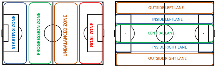
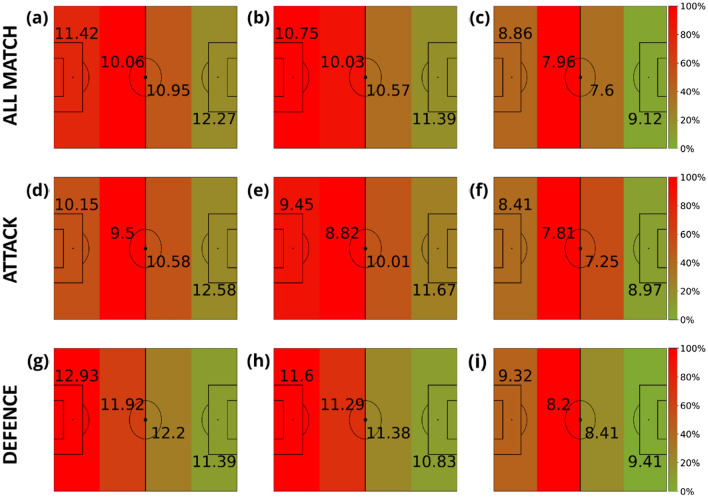
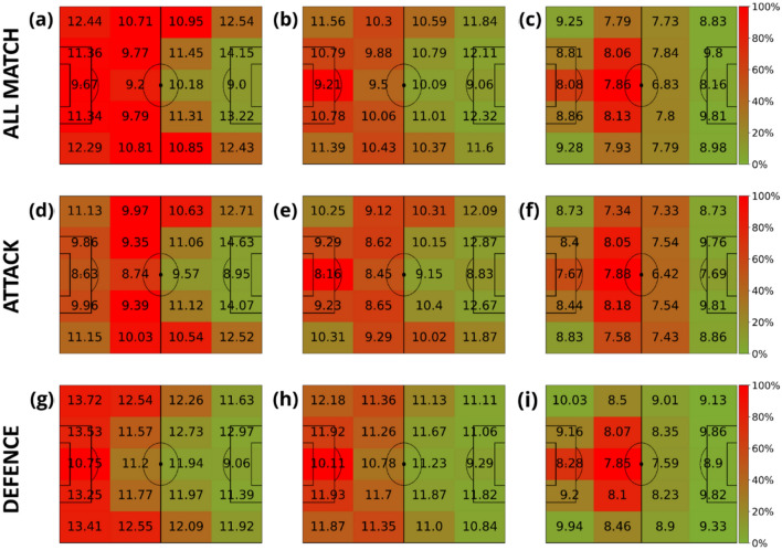
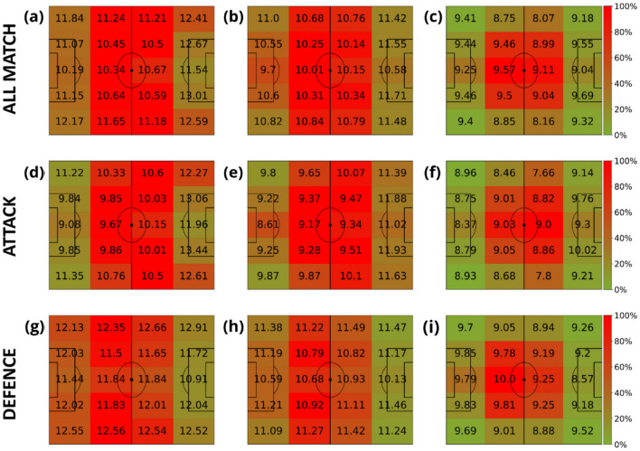
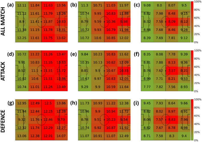
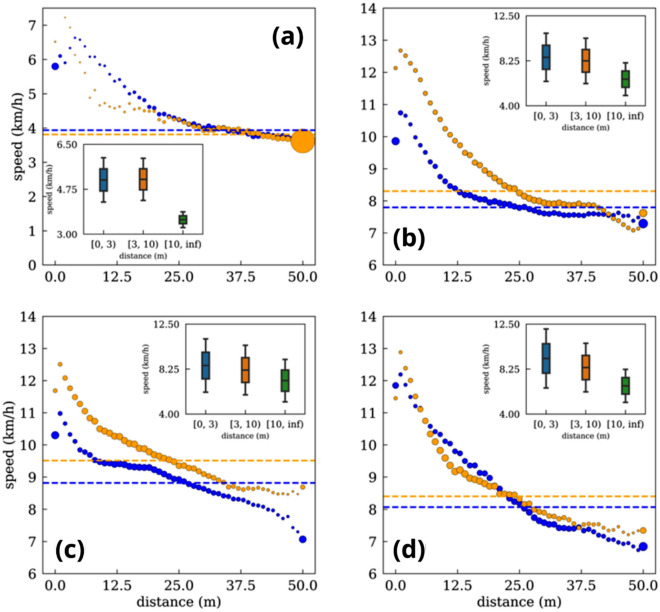
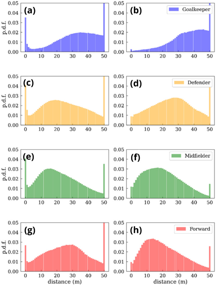
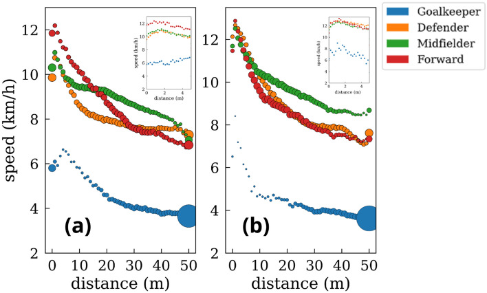
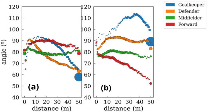
The study analyzes how the magnitude and angle of the speed of soccer players change according to the distance to the ball and the phases of the game, namely the defensive and attacking phases. We observed how the role played in the team (goalkeeper, defender, midfielder, or forward) strongly determines the speed pattern of players. As a general trend, the speed's modulus is incremented as their position is closer to the ball, however, it is slightly decreased when arriving at it. Next, we studied how the angle of the speed with the direction to the ball is related to the distance to the ball and the game phases. We observed that, during the defensive phase, goalkeepers are the players that run more parallel to the ball, while forwards are the ones running more directly to the ball position. Importantly, this behavior changes dramatically during the attacking phase. Finally, we show how the proposed methodology can be used to analyze the speed-angle patterns of specific players to understand better how they move on the pitch according to the distance to the ball.

Keywords: Match analysis; Performance; Player behaviour; Player speed; Soccer; Tracking datasets.

Figure 1

Qualitative description of the player’s speed and angle. The distance to the ball of player $i$ is the modulus of $\overrightarrow{r_i}$, and the angle ${\theta }_i$ is computed using the scalar product between $\overrightarrow{r_i}$ and $\overrightarrow{v_i}$ . In the figure, players $a$ and $b$ run at different speeds, $\overrightarrow{v_a}$ and $\overrightarrow{v_b}$, and different angles, ${\theta }_a$, and ${\theta }_b$, respectively.

Figure 2

Division of the pitch. We considered 2 divisions of the pitch, one regarding the opponent’s goal proximity (left plot) and another with regard to the side lanes (right plot). The former is divided into four regions, while the latter is divided into five regions, each related to a tactical conception of the game. Finally, both divisions are joined into a single one, leading to 4 × 5 pitch divisions (i.e., containing 20 different pitch regions).

Figure 3

Average velocities (km/h) of players in terms of their distance to the ball. The intervals of the distance to the ball were: [0, 3) meters (first column), [3, 10) meters (second column) and (10, inf) meters (last column). Note that the values displayed in each zone are the average velocity of players in that region of the field, and the heatmap colors represent the amount of time these players spent inside each region. This value is normalized by the maximum amount of time obtained at each plot. Each row represents different game phases: the first row contains all phases (attacking and defending phases combined), the second corresponds to the attacking phase, and the third is the defending phase. The divisions are the ones proposed in Fig. 2.

Figure 4

Average velocities (km/h) of players in terms of their distance to the ball. The intervals of the distance to the ball were: [0, 3) meters (first column), [3, 10) meters (second column) and (10, inf) meters (last column). Note that the values displayed in each zone are the average velocity of all the players in that region of the field, and the heatmap colors represent the amount of time these players spent inside each region. This value is normalized by the maximum amount of time obtained at each plot. Each row represents different game phases: the first row contains all phases (attacking and defending phases combined), the second corresponds to the attacking phase, and the third is the defending phase. The divisions are the ones proposed in Fig. 2.

Figure 5

Average velocities (km/h) of players in terms of their distance to the ball. The intervals of the distance to the ball were: [0, 3) meters (first column), [3, 10) meters (second column) and (10, inf) meters (last column). Note that the values displayed in each zone are the average velocity of players in that region of the field, and the heatmap colors represent the amount of time these players spent inside each region. This value is normalized by the maximum amount of time obtained at each plot. Each row represents different game phases: the first row contains all phases (attacking and defending phases combined), the second corresponds to the attacking phase, and the third is the defending phase. In this case, the spatial partition combines the ones proposed at Figs. 3 and 4, leading to a 4 × 5 grid.

Figure 6

Average velocities (km/h) of goalkeepers in terms of their distance to the ball. The intervals of the distance to the ball were: [0, 3) meters (first column), [3, 10) meters (second column) and (10, inf) meters (last column). The heatmap colors represent the normalized amount of time these players spent inside each region. Each row represents different phases of the game: the first row contains all phases, the second corresponds to the attacking phase, and the third is the defending phase.

Figure 7

Average velocities (km/h) of defenders in terms of their distance to the ball. The intervals of the distance to the ball were: [0, 3) meters (first column), [3, 10) meters (second column) and (10, inf) meters (last column). The heatmap colors represent the normalized amount of time these players spent inside each region. Each row represents different game phases: the first row contains all phases, the second corresponds to the attacking phase, and the third is the defending phase.

Figure 8

Average velocities (km/h) of midfielders in terms of their distance to the ball. The intervals of the distance to the ball were: [0, 3) meters (first column), [3, 10) meters (second column) and (10, inf) meters (last column). The heatmap colors represent the normalized amount of time these players spent inside each region. Each row represents different game phases: the first row contains all phases, the second corresponds to the attacking phase, and the third is the defending phase.

Figure 9

Average velocities (km/h) of forwards in terms of their distance to the ball. The intervals of the distance to the ball were: [0, 3) meters (first column), [3, 10) meters (second column) and (10, inf) meters (last column). The heatmap colors represent the normalized amount of time these players spent inside each region. Each row represents different game phases: the first row contains all phases, the second corresponds to the attacking phase, and the third is the defending phase.

Figure 10

Average speed at different distances from the ball. (a) Goalkeepers. (b) Defenders. (c) Midfielders. (d) Forwards. Orange circles indicate the speed averages while defending, and blue points are the speed averages while attacking. The dashed orange line represents the average defending speed, and the blue one is the average attacking speed. The inset shows the speed distributions in the three discrete intervals. The size of the circles for each position is proportional to the time spent at each distance [see Fig. 11 for a more detailed analysis].

Figure 11

Time spent by players at different distances to the ball. For each player role, we plot the probability distribution function (p.d.f.) of the time spent at each distance to the ball. Attacking (a, c, e and g) and defending (b, d, f and h) phases.

Figure 12

Scatter plot of the average speed as a function of the distance to the ball at all game phases. Goalkeepers (blue), defenders (orange), midfielders (green), and forwards (red). The size of the points is proportional to the p.d.f of the time spent at each distance.

Figure 13

Differences in the average speed of the players as a function of the distance to the ball for the (a) attacking and (b) defensive phases. Goalkeepers (blue), defenders (orange), midfielders (green), and forwards (red). The size of the points is proportional to the p.d.f of the time spent at each distance.

Figure 14

Scatter plot of the average angle between the velocity of the players and their distance to the ball vector (see Fig. 1 for details). Goalkeepers (a), defenders (b), midfielders (c), and forwards (d). Blue and orange colors correspond to the attacking and defending phases, respectively. The dashed orange line represents the average angle while defending, while the blue one is the average attacking angle. The size of the points is proportional to the p.d.f of the time spent at each distance.

Figure 15

Scatter plot of the average angle between the velocity of the players and their distance to the ball vector at (a) attacking and (b) defending phases. Goalkeepers (blue), defenders (orange), midfielders (green), and forwards (red). The size of the points for each position is proportional to the p.d.f of the time spent at each distance.

References

1. Aguiar M, Gonçalves B, Botelho G, Lemmink K, Sampaio J. Footballers’ movement behaviour during 2-, 3-, 4- and 5-a-side small-sided games. J. Sports Sci. 2015;33:1259–1266. doi: 10.1080/02640414.2015.1022571. - DOI - PubMed
1. Casamichana D, Castellano J, Calleja-Gonzalez J, San Román J, Castagna C. Relationship between indicators of training load in soccer players. J. Strength Cond. Res. 2013;27:369–374. doi: 10.1519/JSC.0b013e3182548af1. - DOI - PubMed
1. Duarte R, Araujo D, Correia V, Davids K. Sports teams as superorganisms: Implications of sociobioloical models of behaviour for research and practice in team sports performance analysis. Sports Med. 2012;42:633–643. doi: 10.1007/BF03262285. - DOI - PubMed
1. Duarte R, Araujo D, Folgado H, Esteves P, Marques P, Davids K. Capturing complex, non-linear team behaviours during competitivesoccer performance. J. Syst. Sci. Complex. 2013;26:62–72. doi: 10.1007/s11424-013-2290-3. - DOI
1. Ribeiro J, Silva P, Duarte R, Davids K, Garganta J. Team sports performance analysed through the lens of social network theory: Implications for research and practice. Sports Med. 2017;47:1689–1696. doi: 10.1007/s40279-017-0695-1. - DOI - PubMed