When Two Eyes Don't Suffice-Learning Difficult Hyperfluorescence Segmentations in Retinal Fundus Autofluorescence Images via Ensemble Learning

Abstract

Hyperfluorescence (HF) and reduced autofluorescence (RA) are important biomarkers in fundus autofluorescence images (FAF) for the assessment of health of the retinal pigment epithelium (RPE), an important indicator of disease progression in geographic atrophy (GA) or central serous chorioretinopathy (CSCR). Autofluorescence images have been annotated by human raters, but distinguishing biomarkers (whether signals are increased or decreased) from the normal background proves challenging, with borders being particularly open to interpretation. Consequently, significant variations emerge among different graders, and even within the same grader during repeated annotations. Tests on in-house FAF data show that even highly skilled medical experts, despite previously discussing and settling on precise annotation guidelines, reach a pair-wise agreement measured in a Dice score of no more than 63-80% for HF segmentations and only 14-52% for RA. The data further show that the agreement of our primary annotation expert with herself is a 72% Dice score for HF and 51% for RA. Given these numbers, the task of automated HF and RA segmentation cannot simply be refined to the improvement in a segmentation score. Instead, we propose the use of a segmentation ensemble. Learning from images with a single annotation, the ensemble reaches expert-like performance with an agreement of a 64-81% Dice score for HF and 21-41% for RA with all our experts. In addition, utilizing the mean predictions of the ensemble networks and their variance, we devise ternary segmentations where FAF image areas are labeled either as confident background, confident HF, or potential HF, ensuring that predictions are reliable where they are confident (97% Precision), while detecting all instances of HF (99% Recall) annotated by all experts.

Keywords: CSCR; U-Net; ambiguous; annotation; central serous chorioretinopathy; deep learning; ensemble; fundus autofluorescence; hyperfluorescence; image analysis; inter-observer variability; intra-observer variability; reduced autofluorescence; retinal; segmentation; ternary.

Figure 3

Generating a segmentation prediction (yellow HF, rest no HF) and a ternary prediction (green confident HF, yellow potential HF, rest no HF) from the proposed segmentation ensemble. Details for the generation of the ternary segmentation output are given in Figure 5.

Figure A1

HF segmentation performance in relation to the size of annotated HF for the ensemble.

Figure A2

Comparison of HF annotation sizes for the test and validation dataset. The height of the curve for any given annotation size on the abscissa indicates the ratio of smaller annotations in the dataset. We see that the test dataset contains more extreme (very small and very large) HF annotations than the validation dataset.

Figure A3

The ensemble’s segmentation score in regard to the annotation size. The height of the curve for any point on the abscissa indicates the $mDc{S}_{AE}$ score the ensemble would obtain if we only considered the images with $larger$ HF annotations. The data shows that lower test scores are caused mainly by bad segmentations for a few images with very large HF area (compare Figure A1). The data also show that segmentation scores are generally high but suffer from the set of images with very small annotations.

Figure A4

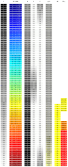
The HyperExtract [15] color conversion table. Given are the image’s grayscale intensity values I after preprocessing (with step size 3 for readability), the resulting JET color map RGB values and resulting HSV values. HSV values are given in the ranges of the OpenCV library [66], as [15] explicitly mention the usage of the OpenCV inRange() function. $p\left(I\right)$ denotes the probability of a pixel with intensity I after preprocessing to be HF in our validation dataset. The column HE denotes pixels that will be classified as HF by our adapted HyperExtract method. The column ${\mathit{HE}}_{orig}$ denotes pixels that will be classified as different stages of HF by the original extraction ranges given in [15].

Figure A5

Analysis of our validation dataset in regard to the relationship of pixel intensity I after preprocessing and the probability of belonging to an HF area. The height of the gray bars (from 0) depicts the relative number of appearances of pixels with a given intensity I. The height of the yellow bars depicts the relative number of pixels with this intensity belonging to HF. Pixels with intensity 0 are omitted for better readability.

Figure A6

Validation and test Dice scores for the HyperExtract baseline over different thresholds ${\mu }_{HE}$ . From the data shown in Figure A5, we calculate for each pixel intensity I its probability $p\left(I\right)$ of belonging to HF (as depicted in Figure A4). Only pixels with $p\left(I\right)>={\mu }_{HE}$ are segmented as HF. Optimal results for the validation and test dataset are achieved with ${\mu }_{HE}=0.07$ and ${\mu }_{HE}=0.06$ , respectively. The dashed horizontal lines show the results achieved with the original extraction ranges given in [15].

Figure A7

(Images are best viewed zoomed in). HF segmentations on the single-annotation validation set for HyperExtract [15] both for our adapted method (d) and the method with the original extraction ranges (e). Predictions of our full ensemble (c) and the expert annotations (b) are given for comparison. The top row depicts the same image, as shown on the top in Figure 10, the bottom row shows an image, where the H-Extract achieves a $DcS=0.255$ very close to its mean $DcS$ on the validation set (=0.251, see Table 3).

Figure A8

(Images are best viewed zoomed in). HF ternary predictions on the single-annotation validation set for the diffusion model baseline [31] (c) with 10 predictions per image plus mean (d) and variance (e) outputs. The top row shows the same image as on the top of Figure 10 and Figure A7. Here, the diffusion models in 10 predictions dos not predict anything. The middle row shows the same eye as the top but at a later date. Here, the diffusion model reaches $recal{l}_{C\to CP}=0.466$ close to its mean on the validation set (=0.456, see Table 3). The bottom row shows a case where the diffusion model reaches a very good score of $recal{l}_{C\to CP}=0.952$ .

Figure 1

From the multiple expert’s HF annotations (yellow in (a)) we are able to generate segmentations for confident HF (green), where HF has been seen by all experts and segmentations for potential HF (yellow in (b–d)) where HF has been seen by some experts (see Figure 5 in Section 4.1). When comparing the expert’s ternary (b) to the ternary generated from a single U-Net’s prediction confidence (c) as well as the ternary generated from the mean prediction confidence and its variance of our proposed segmentation ensemble (d), we see that not only is the ensemble’s overall segmentation more accurate; the ensemble’s confident HF prediction more accurately aligns with the expert’s confident HF, whereas the single U-Net displays typical overconfidence on almost all segmented areas. Please note that the expert’s RA annotations are not shown for reasons of clarity.

Figure 2

(Images are best viewed zoomed in). To align the subset of images (a) with fine annotations by Expert 1 (b) with the coarser annotations performed for the remaining images as in (d), we apply morphological closing ( $15\times 15$ pixels kernel) on the segmentation masks for HF (yellow) and RF (not seen here), while ignoring granular hyper autofluorescence (violet) and granular hypo autofluorescence (blue). Should a pixel afterward belong to both the HF and the RF mask, it becomes part of the HF mask. The resulting aligned annotation is shown in (c).

Figure 4

Synthetic example to show for two predictions (red and green in a,d) the difference between the Dice score $DcS$ (a,d) and the adjusted area error Dice score $Dc{S}_{AE}$ for ${\mu }_{EE}=60$ px (c,f) (TP green, EE blue, AE red) generated from the distance maps (b,e) (warmer colors indicate higher distance from agreement TP). The prediction shown in red stays the same between the top and bottom case. The prediction shown in green changes, such that on the top it only detects one red area, whereas on the bottom it detects both red areas (though the larger area with less overlap). In the context of clinical HF detection, the green prediction depicted in the bottom row is preferable to the green prediction depicted on top despite identical $DcS$ values. The $Dc{S}_{AE}$ metric reflects that.

Figure 5

Ternary task: categorizing pixels into P (potential HF), C (confident HF), and B (background) depending on the input type, the general idea being that a high variance indicates P, whereas a low variance indicates C or B, depending on the mean. If no variance is available, two thresholds are applied to the prediction value p. Hence, for a single annotation no pixel can be categorized as P.

Figure 6

(Images are best viewed zoomed in). HF segmentation predictions (top row), ternary predictions (second row), prediction means (third row), and variances (bottom row) for an image in the validation dataset. For the ternary task, yellow indicates P (potential predictions) and green C (confident predictions). Sub-Ens_m depicts the prediction of a sub-ensemble with m networks.

Figure 7

(Images are best viewed zoomed in). HF prediction results on the test set for our proposed ensembles (d,e) and a single segmentation U-Net (c). Images (a) where chosen such that the results for Sub-Ens₁₀ (0.67 $recal{l}_{CP\to C}$ top, 0.59 $recal{l}_{CP\to C}$ middle, 0.66 $mDc{S}_{AE}$ bottom) are close to the mean results (0.63 $recal{l}_{CP\to C}$ , 0.63 $mDc{S}_{AE}$ ) shown in Table 5. Please note that the upper two rows show results and annotations (b) for the ternary task, while the bottom row shows results and annotations (b) for the segmentation task.

Figure 8

The ratio of $AE$ compared to $FP+FN$ (i.e., all pixels labeled differently) among the five available expert annotations over nine FAF images for different ${\mu }_{EE}$ . The ratio of $EE$ is the inverse of the curve depicted here since $EE+AE=FP+FN$ .

Figure 9

Comparison of experts annotations (a–e) and ensemble predictions (f) for HF (yellow) and RA (red). Expert 1* denotes segmentations of Expert 1 several months after the original annotations.

Figure 10

(images are best viewed zoomed in). HF ternary performance for different ensembles (c–f) and the single U-Net baseline (b) on two images. “experts” (a) denotes the ternary ground truth created from all 5 available expert annotations.

Figure 11

Segmentation scores (a,b) and ternary scores (c,d) on the test set of 60 images with HF (yellow) and 55 images with RA (red) for the proposed sub-ensemble sampled by solving the MDP and the sub-ensemble baselines sampled either by selecting the n best performing networks (n best) or sampling in equal steps (n steps) based on the segmentation performance (i.e., worst, median, and best for $n=3$ ). Scores are shown in relation to the number n of networks in the sub-ensemble.

References

1. Yung M., Klufas M.A., Sarraf D. Clinical applications of fundus autofluorescence in retinal disease. Int. J. Retin. Vitr. 2016;2:1–25. doi: 10.1186/s40942-016-0035-x. - DOI - PMC - PubMed
1. Pichi F., Abboud E.B., Ghazi N.G., Khan A.O. Fundus autofluorescence imaging in hereditary retinal diseases. Acta Ophthalmol. 2018;96:e549–e561. doi: 10.1111/aos.13602. - DOI - PubMed
1. Schmitz-Valckenberg S., Pfau M., Fleckenstein M., Staurenghi G., Sparrow J.R., Bindewald-Wittich A., Spaide R.F., Wolf S., Sadda S.R., Holz F.G. Fundus autofluorescence imaging. Prog. Retin. Eye Res. 2021;81:100893. doi: 10.1016/j.preteyeres.2020.100893. - DOI - PubMed
1. Sparrow J.R., Duncker T., Schuerch K., Paavo M., de Carvalho Jr J.R.L. Lessons learned from quantitative fundus autofluorescence. Prog. Retin. Eye Res. 2020;74:100774. doi: 10.1016/j.preteyeres.2019.100774. - DOI - PMC - PubMed
1. Schmidt-Erfurth U., Sadeghipour A., Gerendas B.S., Waldstein S.M., Bogunović H. Artificial intelligence in retina. Prog. Retin. Eye Res. 2018;67:1–29. doi: 10.1016/j.preteyeres.2018.07.004. - DOI - PubMed