LinG3D: visualizing the spatio-temporal dynamics of clonal evolution

Abstract

Background: Cancers are spatially heterogenous, thus their clonal evolution, especially following anti-cancer treatments, depends on where the mutated cells are located within the tumor tissue. For example, cells exposed to different concentrations of drugs, such as cells located near the vessels in contrast to those residing far from the vasculature, can undergo a different evolutionary path. However, classical representations of cell lineage trees do not account for this spatial component of emerging cancer clones. Here, we propose routines to trace spatial and temporal clonal evolution in computer simulations of the tumor evolution models.

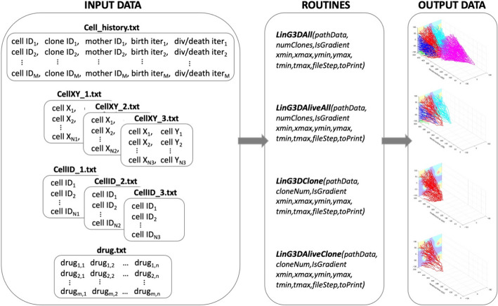
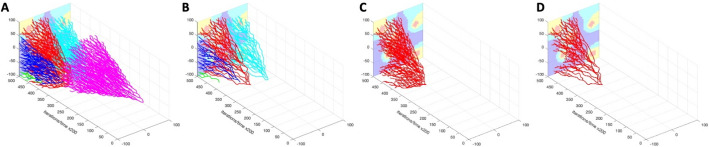
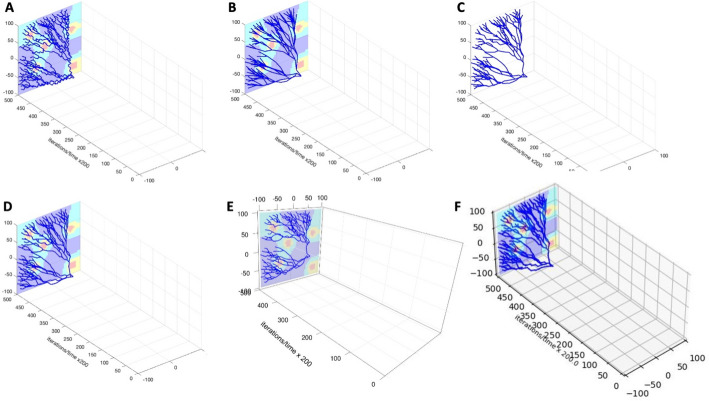
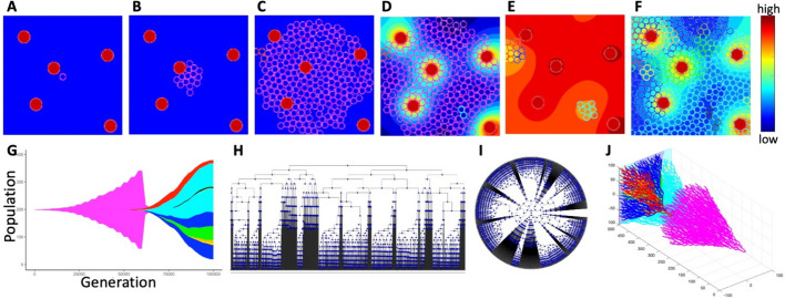
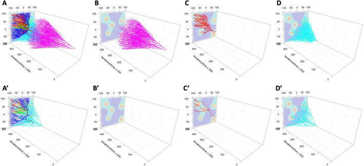
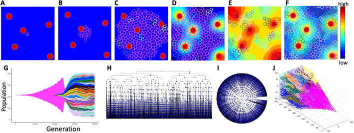
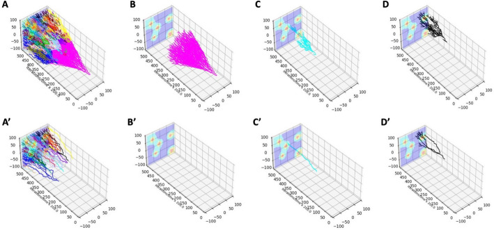
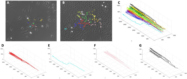
Results: The LinG3D (Lineage Graphs in 3D) is an open-source collection of routines (in MATLAB, Python, and R) that enables spatio-temporal visualization of clonal evolution in a two-dimensional tumor slice from computer simulations of the tumor evolution models. These routines draw traces of tumor clones in both time and space, and may include a projection of a selected microenvironmental factor, such as the drug or oxygen distribution within the tumor, if such a microenvironmental factor is used in the tumor evolution model. The utility of LinG3D has been demonstrated through examples of simulated tumors with different number of clones and, additionally, in experimental colony growth assay.

Conclusions: This routine package extends the classical lineage trees, that show cellular clone relationships in time, by adding the space component to show the locations of cellular clones within the 2D tumor tissue patch from computer simulations of tumor evolution models.

Keywords: 3D visualization; Lineage trees; Mathematical modeling of tumor evolution; Spatial clone distribution.

Fig. 1

Architecture of the LinG3D routine package. The specified four types of text files are required as the input data for each of the four routines within the LinG3D package; each routine generates a graphical result as an output data

Fig. 2

Examples of outcomes from four LinG3D routines. A a 3D full lineage tree with all cells and clones (LinG3DAll routine); B a 3D lineage tree with all surviving cells (LinG3DAliveAll routine); C a 3D lineage tree with all cells for a single clone (LinG3DClone routine); D a 3D lineage tree with all surviving cells in one clone (LinG3DAliveClone routine). In all examples, the drug distribution is shown in the background with concentrations from high to low represented by: red-yellow-cyan-blue

Fig. 3

User-specified parameters and computational language options. A A 3D lineage tree of surviving cells for one clone (LinG3DAliveClone) drawn with data sampling parameter fileStep = 250; B The same lineage tree drawn with data sampling parameter fileStep = 5000; C The same lineage tree drawn with no background IsGradient = 0 and with data sampling parameter fileStep = 2500. D–F 3D lineage trees of the same single clone of surviving cells drawn with routines implemented in MATLAB (D), R (E), and Python (F), respectively (fileStep = 2000)

Fig. 4

Evolution of a 9-clone tumor. Tumor growth simulated using tumorGrowth_example1 with a parameter ${\mathcal{P}}^{\mathit{mut}}$=0.005: A an initial tumor cell (pink, iteration 0); B a growing cluster of non-mutated tumor cells (pink, iteration 18,000); C the emergence of the first mutated cell (red, top left edge, iteration 56,500); D the beginning of drug injection (second mutated clone in cyan, iteration 60,250); E drug-induced cell death (iteration 63,250); F the final configuration with 9 cellular clones (iteration 100,000). The color bar represents the drug concentration. G the corresponding tumor jellyfish evolution graph (ggmuller routine [2]); Clone colors correspond to cell colors in (A–F). H, I a classical lineage tree showing the relationship between mother and daughter cells in square and radial configuration (phytree routine [5]); J the corresponding full 3D lineage tree (our LinG3DAll routine)

Fig. 5

3D lineage trees of individual clones drawn with R routines. For each clone (denoted by a different color), the top row shows the 3D lineage tree with all cells belonging to that clone (A LinG3DAll and B–D LinG3DClone routines), while the bottom row includes only the cells that survived to the end of the simulation (A’ LinG3DAliveAll and B’–D’ LinG3DAliveClone routines). B–B’ initial clone #0; C–C’ mutated clone #1; D–D’ mutated clone #2

Fig. 6

Evolution of a 147-clone tumor. Tumor growth simulated using tumorGrowth_example2 with a parameter ${\mathcal{P}}^{\mathit{mut}}$=0.05: A an initial tumor cell (pink, iteration 0); B a growing cluster of non-mutated tumor cells (pink, iteration 18,000); C ten mutated cells have already emerged (multiple colors, iteration 56,500); D the beginning of drug injection (iteration 60,250); E drug-induced cell death (iteration 63,250); F the final configuration with 147 cellular clones (iteration 100,000); the color bar represents the drug concentration. G the corresponding tumor evolution graph (ggmuller routine [2]); clone colors correspond to cell colors in (A–F). H, I classical lineage trees showing the relationship between mother and daughter cells in square and radial configurations (phytree routine [5]). J the corresponding full 3D lineage tree (our LinG3DAll routine)

Fig. 7

3D lineage trees of individual clones drawn with Python routines. For each clone (denoted by a different color), the top row shows the 3D lineage tree with all cells belonging to that clone (A LinG3DAll and B–D LinG3DClone routine), while the bottom row includes only the cells that survived to the end of the simulation (A’ LinG3DAliveAll and B’–D’ LinG3DAliveClone routine). B–B’ initial clone #0; C–C’ mutated clone #2; D–D’ mutated clone #5

Fig. 8

3D lineage trees (MATLAB routines) for individual clones identified in an experimental assay. A, B the initial and final frames from a bright field time-lapse microscopy of a growing cell colony with 10 different clones indicated by different colors. C 3D lineage trees for all ten cellular clones (LinG3DAll); D–G 3D lineage trees for all cells in four selected cellular clones (LinG3DClone); each tree color corresponds to cells’ colors in (A and B)

References

1. Nowell PC. The clonal evolution of tumor cell populations. Science. 1976;194(4260):23–28. doi: 10.1126/science.959840. - DOI - PubMed
1. Noble R, Burri D, Le Sueur C, Lemant J, Viossat Y, Kather JN, et al. Spatial structure governs the mode of tumour evolution. Nat Ecol Evol. 2021;6(2):207–217. doi: 10.1038/s41559-021-01615-9. - DOI - PMC - PubMed
1. Miller CA, McMichael J, Dang HX, Maher CA, Ding L, Ley TJ, et al. Visualizing tumor evolution with the fishplot package for R. BMC Genomics. 2016;17(1):880. doi: 10.1186/s12864-016-3195-z. - DOI - PMC - PubMed
1. Gatenbee CD, Schenck RO, Bravo RR, Anderson ARA. EvoFreq: visualization of the evolutionary frequencies of sequence and model data. BMC Bioinform. 2019;20(1):710. doi: 10.1186/s12859-019-3173-y. - DOI - PMC - PubMed
1. MATLAB. phytree routine documentation and examples. 2021 https://www.mathworks.com/help/bioinfo/ref/phytree.html