Multiscale selection in spatially structured populations

Abstract

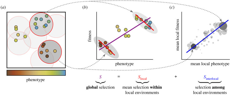
The spatial structure of populations is key to many (eco-)evolutionary processes. In such cases, the strength and sign of selection on a trait may depend on the spatial scale considered. An example is the evolution of altruism: selection in local environments often favours cheaters over altruists, but this can be outweighed by selection at larger scales, favouring clusters of altruists over clusters of cheaters. For populations subdivided into distinct groups, this effect is described formally by multilevel selection theory. However, many populations do not consist of non-overlapping groups but rather (self-)organize into other ecological patterns. We therefore present a mathematical framework for multiscale selection. This framework decomposes natural selection into two parts: local selection, acting within environments of a certain size, and interlocal selection, acting among them. Varying the size of the local environments subsequently allows one to measure the contribution to selection of each spatial scale. To illustrate the use of this framework, we apply it to models of the evolution of altruism and pathogen transmissibility. The analysis identifies how and to what extent ecological processes at different spatial scales contribute to selection and compete, thus providing a rigorous underpinning to eco-evolutionary intuitions.

Keywords: Price’s equation; altruism; evolution; pathogen transmissibility; self-organization; spatial structure.

Figure 1.

Illustration of the spatial decomposition of selection. (a) Spatially structured population of individuals that differ in some phenotypic characteristic. Local environments are defined as circular areas with a given radius. (b) Example of global and local selection pointing in different directions. The covariance between phenotype and fitness within all local environments is negative (i.e. local selection is negative), as evident from the negative slopes of the red regression lines; nevertheless, the global covariance between phenotype and fitness is positive (i.e. global selection is positive), as apparent from the positive slope of the purple regression line. This is an example of Simpson’s paradox. (c) The negative local selection is counteracted by a positive covariance between the mean phenotype and mean fitness of local environments (see the blue regression line). Local environments are weighted by their population density and mean fitness (size of points). This covariance represents the selection among environments, i.e. the interlocal selection.

Figure 2.

Evolution of altruism. (a) Cartoon illustration of the model. Both resource competition and altruism are local processes. The range of resource competition, σ_rc, is larger than the range of altruism, σ_a. (b) Snapshot of part of the simulation plane (see electronic supplementary material, movie S1 for dynamics). The hexagonal lattice constant of the emerged colony pattern is a = 8.4σ_a. The green arrow indicates a colony fission event. (c) Mean level of altruism over time, in a population that is well-mixed (grey) or spatially structured (blue). (d) Cumulative selection (purple) and its spatial decomposition (red and blue) as a function of the length scale r of local environments, measured over the first 40 000 simulation time steps (3200 generations; blue-shaded area in (c)). (e) Contribution to cumulative selection of different length scales measured over the first 40 000 simulation time steps (calculated as the derivative of S_local(r) in (d) with respect to r; see equation (2.2)). The red area indicates a negative contribution to selection, green a positive contribution. (f) Spatial decomposition of selection differential S at evolutionary equilibrium. S_local(r) and S_interlocal(r) were calculated as averages over the last 40 000 simulation time steps (3200 generations) of the simulation (grey-shaded area in (c)).

Figure 3.

Evolution of pathogen transmissibility. (a) Cartoon illustration of the model. (b) Snapshot of part of the simulation lattice for two different values of the reproduction rate of susceptible individuals, γ. Susceptible individuals are plotted in grey, infected individuals are coloured based on the transmissibility of the pathogen they carry. See electronic supplementary material, movies S2 and S3 for dynamics. (c) Mean transmissibility of the pathogen over time in populations that are well-mixed (grey) or spatially structured (blue) for default parameter settings (γ = 0.05). Two spatially structured simulations are shown which were initialized with different transmissibility values. Time is measured in generations, with generation time defined as mean lifespan of susceptible individuals. (d) Spatial decomposition of cumulative selection in the default simulation (γ = 0.05, initial transmissibility = 5, lighter blue line in c) in the early part of the simulation, where selection on transmissibility is positive (S > 0). S, S_local and S_interlocal were summed over the first 10 000 simulation time steps (500 generations). (e) Contribution of varying length scales to the cumulative selection over the first 500 generations, calculated as the derivative of S_local(r). (f) Spatial decomposition of the selection differential at evolutionary equilibrium. For both values of γ, S_local and S_interlocal were now calculated as the mean value over 10 000 simulation time steps between time = 9500 and 10 000 generations. We define the critical scale of selection, r_C, as the length scale at which the contribution to selection switches from positive to negative (i.e. where s(r) = dS_local/dr switches sign). (g) Critical scale of selection, r_C, plotted against size of the emerged patterns for different values of the susceptible reproduction rate γ. Pattern size was determined using the pairwise correlation function (see electronic supplementary material, text).

References

1. Lion S, Baalen M. 2008. Self-structuring in spatial evolutionary ecology. Ecol. Lett. 11, 277-295. (10.1111/j.1461-0248.2007.01132.x) - DOI - PubMed
1. Stacy A, McNally L, Darch SE, Brown SP, Whiteley M. 2016. The biogeography of polymicrobial infection. Nat. Rev. Microbiol. 14, 93-105. (10.1038/nrmicro.2015.8) - DOI - PMC - PubMed
1. Nadell CD, Drescher K, Foster KR. 2016. Spatial structure, cooperation and competition in biofilms. Nat. Rev. Microbiol. 14, 589-600. (10.1038/nrmicro.2016.84) - DOI - PubMed
1. Yanni D, Márquez-Zacarías P, Yunker PJ, Ratcliff WC. 2019. Drivers of spatial structure in social microbial communities. Curr. Biol. 29, R545-R550. (10.1016/j.cub.2019.03.068) - DOI - PubMed
1. Dal Co A, van Vliet S, Kiviet DJ, Schlegel S, Ackermann M. 2020. Short-range interactions govern the dynamics and functions of microbial communities. Nat. Ecol. Evol. 4, 366-375. (10.1038/s41559-019-1080-2) - DOI - PubMed
LinkOut - more resources