Information content and optimization of self-organized developmental systems

Abstract

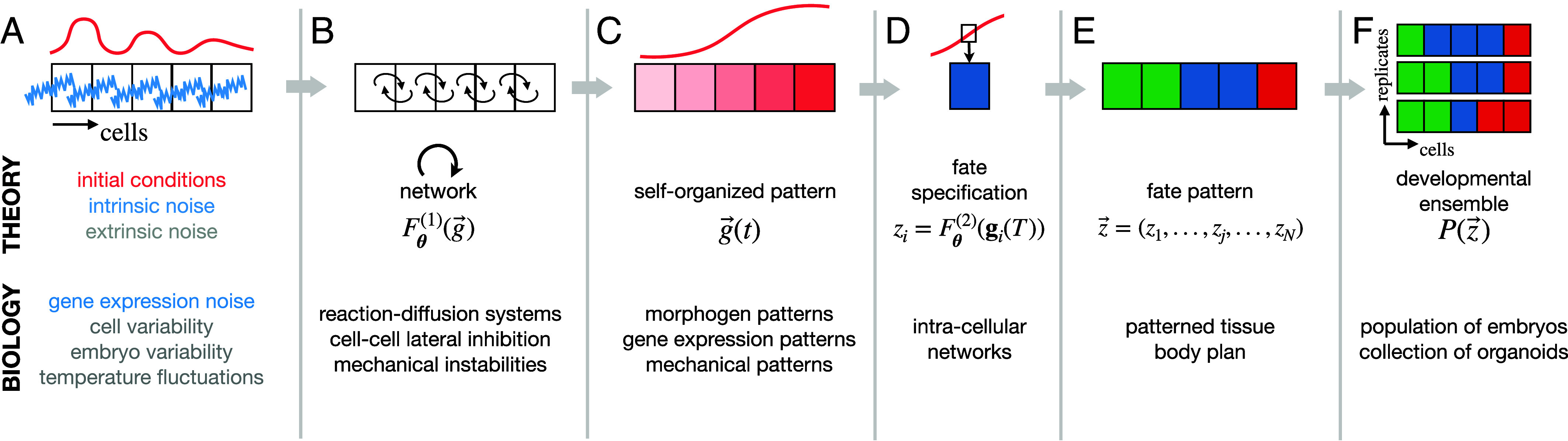
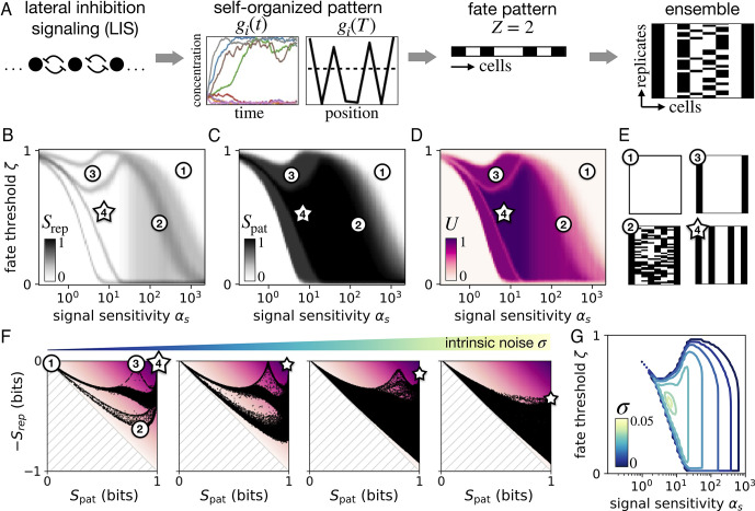
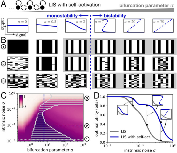
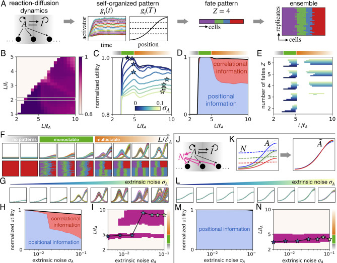
A key feature of many developmental systems is their ability to self-organize spatial patterns of functionally distinct cell fates. To ensure proper biological function, such patterns must be established reproducibly, by controlling and even harnessing intrinsic and extrinsic fluctuations. While the relevant molecular processes are increasingly well understood, we lack a principled framework to quantify the performance of such stochastic self-organizing systems. To that end, we introduce an information-theoretic measure for self-organized fate specification during embryonic development. We show that the proposed measure assesses the total information content of fate patterns and decomposes it into interpretable contributions corresponding to the positional and correlational information. By optimizing the proposed measure, our framework provides a normative theory for developmental circuits, which we demonstrate on lateral inhibition, cell type proportioning, and reaction-diffusion models of self-organization. This paves a way toward a classification of developmental systems based on a common information-theoretic language, thereby organizing the zoo of implicated chemical and mechanical signaling processes.

Keywords: development; information theory; self-organization; signaling networks.

Fig. 1.

Entropy and information plane characterize self-organization outcomes. (A) Schematic of the statistical approach to cell fate patterns, in which an assembly of cells of different cell fates is represented as a vector of discrete fates (Left). Cells may have different shapes, sizes, and may be placed in complex, not necessarily one-dimensional, spatial arrangements. Sampling from the developmental ensemble $P(\overrightarrow{z})$ results in a list of replicates (Middle). The ensemble is characterized by the distribution of fates $P_z(z)$ pooled across systems and positions; and the marginal distribution $P_i(z_i)$ at each position (Right). (B–E) Examples of ensembles, their entropy values, and information content. (F) Entropy plane spanned by the patterning and reproducibility entropies. (G) Information plane spanned by the PI and correlational information (CI) contributions to the utility. (H) Overview of the three key entropic quantities, and the three information quantities obtained by combinations of the entropies.

Fig. 2.

Cell fate patterning processes. We describe cell fate patterning as a sequence of steps, shown as a schematic (Top), with the corresponding description in our theoretical approach (Middle), and possible biological implementations (Bottom). (A) The system is subject to various sources of stochasticity, including intrinsic noise and extrinsic noise across cells or replicates. The dynamics can also start with randomness in initial conditions. (B) The cells subsequently signal to each other through the signaling network determined by the dynamical systems specified by Eq. 13. (C) This communication establishes self-organized patterns $\overrightarrow{g}(t)$. (D) Each cell autonomously interprets the patterning concentrations at readout time $T$ to decide its fate $z_i$. (E) Fate decisions of all cells yield the fate pattern of one replicate, $\overrightarrow{z}$. (F) A large number of replicates constitutes the developmental ensemble $P(\overrightarrow{z})$.

Fig. 3.

Optimal patterning in a minimal stochastic lateral inhibition system. (A) The production of chemical $g$ in each cell is subject to inhibition by neighboring cells with a sensitivity parameter ${\alpha }_s$. We simulate $N=8$ cells in 1D with nearest neighbor interactions and closed boundary conditions. As time unfolds, symmetry is broken with some cells having a high and some cells a low concentration of $g$. These concentrations are thresholded with threshold $\zeta$ at readout time $T$ into $Z=2$ cell fates (depicted with black and white in the developmental ensemble). (B–D) Reproducibility entropy, patterning entropy, and utility, respectively, as a function of ${\alpha }_s$ and $\zeta$, with fixed $\sigma =0.01$. Numbers (1)–(4) denote example ensembles shown in panel E. (E) Depictions of four developmental ensembles: no patterning (1), maximally irreproducible ensemble (2), boundary cells only (3), and reproducible alternating patterning (4). (F) Visualization of patterning outcomes in entropy planes for four increasing intrinsic noise levels ($\sigma =\{0.001,0.01,0.05,0.1\}$). Each of the ${10}^5$ dots corresponds to a developmental ensemble defined by a random draw of its parameters $\mathit{\theta }=\{{\alpha }_s,\zeta \}$. (G) High-utility regions in parameter space, defined as $U(\mathit{\theta })>0.99U({\mathit{\theta }}^{\ast })$, for various noise levels $\sigma$ (color-coded).

Fig. 4.

Optimal patterning in a stochastic lateral inhibition system with self-regulation. (A) Nullclines of Eq. 14 as a function of the bifurcation parameter $\alpha$. Solid and dotted lines correspond to stable and unstable fixed points, respectively. The dashed line between panels indicates the onset of bistability at critical ${\alpha }_{\mathrm{c}}=4$. (B) Developmental ensembles for different bifurcation parameter values and nullclines as shown in A. Rows (1)–(3) correspond to three intrinsic noise levels $\sigma =\{0.001,0.01,0.4\}$. Gray frames indicate the optimal parameter ranges at each noise level, as in C. (C) Utility as a function of $\alpha$ and $\sigma$. Optimal parameter range for $\alpha$ for each value of $\sigma$ is indicated by the hatched region, defined as those values of $\alpha$ that have at least 90% of the maximum utility at each noise level. The blue dashed line indicates the onset of bistability at critical ${\alpha }_{\mathrm{c}}=4$. (D) Utility of optimal LIS models without (gray) and with (blue) self-regulation, as a function of noise. For each noise level, all parameters of both LIS models were optimized independently. Insets show optimal response curves of both models at three example noise levels. All panels are plotted with optimized thresholds ${\zeta }^{\ast }$.

Fig. 5.

Optimization of cell-type proportioning and sorting. (A) Schematic of an all-to-all inhibition network with $N=8$ cells, including self-activation in each cell (interactions shown for a single focal cell). Eq. 14 with $f(g_i,s_i)=\alpha (g_i-s_i)$ is used. (B) Developmental ensembles based on independent (binomial) cell fate decisions with equal probability $P=0.5$ for both fates (Top, gray); or on proportioning mechanism of panel A with $\alpha =3,\sigma =0.15$ (Bottom, green). (C) Proportioning distribution $P(N_k)$ of the number of black cells $N_k$ per replicate, for the binomial ensemble (gray line) and the proportioning mechanism (green). (D) PI, CI, and $U$ for the proportioning mechanism. The red dashed line indicates the maximum possible CI for a proportioning process, ${\mathrm{CI}}_{\max }={log}_{2}Z-\frac{1}{N}{log}_2[N!/{(N/Z)}^Z]$ (assuming $N$ is divisible by $Z$, SI Appendix). (E) Utility as a function of the bifurcation parameter $\alpha$ for varying intrinsic noise level $\sigma$ (color bar). The blue dashed line indicates ${\alpha }_{\mathrm{c}}$; the red dashed line indicates ${\mathrm{CI}}_{\max }$. (F) Utility as a function of $\sigma$ with optimally chosen $\alpha$ at each noise level. Different grayscale curves are computed for different values of readout time $T$ (color bar). (G) Schematic of the cell sorting process: cells in each replicate swap places until all black cells are on the Right. (H) Developmental ensembles obtained by noise-free sorting of the ensembles in B. (I) PI as a function of intrinsic noise in the initial proportioning process, obtained after noise-free sorting of the ensembles in F. Blue dashed line: lower bound on PI obtained by sorting a binomial ensemble (SI Appendix). Optimized thresholds ${\zeta }^{\ast }$ are used throughout.

Fig. 6.

Optimal patterning in a stochastic activator–inhibitor system. (A) Schematic of the cell fate patterning process in the activator–inhibitor system. Fate patterns are generated by thresholding the activator profile using a set of thresholds $\{{\zeta }_1,...,{\zeta }_{Z-1}\}$ for $Z$ fates. (B) Normalized utility $U/{log}_{2}Z$ as a function of the activator and inhibitor diffusive length scales (${\sigma }_A=0$). (C) Normalized utility as a function of $L/{\ell }_A$ with $L/{\ell }_I=2$, corresponding to the gray rectangle marked in B, for increasing extrinsic noise magnitude ${\sigma }_A$ using fixed $Z=4$. Shaded bars at the top correspond to the stability regimes indicated in F. Stars denote maximal utility solutions at each noise level. (D) PI and CI contributions to the utility as a function of $L/{\ell }_A$ (${\sigma }_A=0$). (E) Top 1% utility parameter regions as a function of ${\sigma }_A$ (color bar in C) and $Z$. (F) Activator profiles (Top) and fate patterns (Bottom) as a function of $L/{\ell }_A$ with $L/{\ell }_I=2$ (${\sigma }_A=0.05$). (G) Activator profiles as a function of increasing ${\sigma }_A$. For each noise level, $L/{\ell }_A$ is chosen optimally, corresponding to stars in C. (H) PI and CI contributions to the utility of the optimal patterns in G as a function of ${\sigma }_A$. (I) Top 1% utility parameter regions as a function of $L/{\ell }_A$ and ${\sigma }_A$. Stars correspond to the maximal utility solutions in C. (J) Schematic of the network with an additional normalizer species $N$. (K) Example profiles of the activator (Left, solid), normalizer (Left, dashed), and normalizer-corrected profiles (Right). Twenty samples are shown in thin gray lines, with three examples highlighted in blue, green, and red. (L) Normalizer-corrected profiles $\tilde{A}$ for optimal parameter values of $L/{\ell }_A$ as a function of increasing extrinsic noise level ${\sigma }_A$. (M) PI and CI contributions to the utility of the optimal normalizer-corrected profiles as a function of noise level. (N) Top 1% utility parameter regions of the normalizer network as a function of $L/{\ell }_A$ and ${\sigma }_A$. Throughout this example, we use a dimensionless parameterization, with the free parameters held fixed at ${\alpha }_A{\beta }_I/({\beta }_A{\alpha }_I)=0.5$ and $h=5$. We align activator profiles such that maxima are located at $x=L$ and use optimized thresholds. See SI Appendix for a similar analysis with varying intrinsic noise.

Fig. 7.

Classification of self-organized systems in information space. (A) Schematic of developmental stages of three self-organized developmental systems: in vitro intestinal organoids (Top), the early mammalian embryo at the blastocyst stage (Middle), and in vitro 3D gastruloids (Bottom). (B) Hypothesized trajectory in the information plane: initial nonpatterned stages have no information (1), intermediate stages give rise to CI (2), and final stages establish reproducible fate patterns with high PI (3).

References

1. Wolpert L., Positional information and the spatial pattern of cellular differentiation. J. Theor. Biol. 25, 1–47 (1969). - PubMed
1. Jukam D., Shariati S. A. M., Skotheim J. M., Zygotic genome activation in vertebrates. Dev. Cell 42, 316–332 (2017). - PMC - PubMed
1. Gregor T., Tank D. W., Wieschaus E. F., Bialek W., Probing the limits to positional information. Cell 130, 153–164 (2007). - PMC - PubMed
1. Dubuis J. O., Tkacik G., Wieschaus E. F., Gregor T., Bialek W., Positional information, in bits. Proc. Natl. Acad. Sci. U.S.A. 110, 16301–16308 (2013). - PMC - PubMed
1. Petkova M. D., Tkačik G., Bialek W., Wieschaus E. F., Gregor T., Optimal decoding of cellular identities in a genetic network. Cell 176, 844–855.e15 (2019). - PMC - PubMed
LinkOut - more resources