Modeling spatial evolution of multi-drug resistance under drug environmental gradients

Abstract

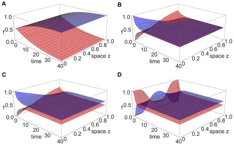
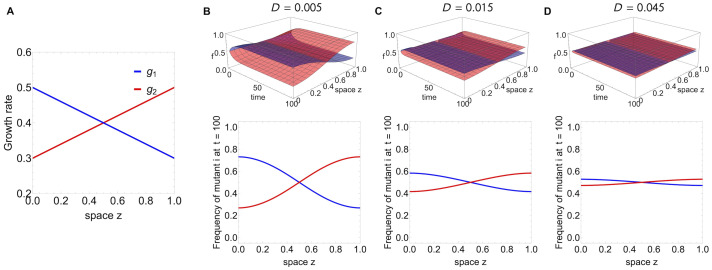
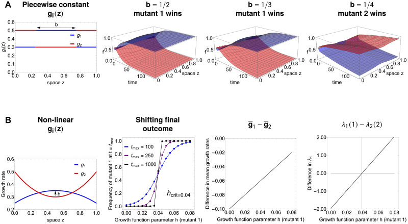
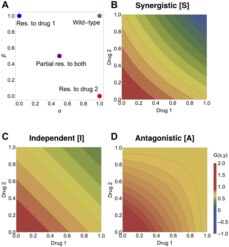
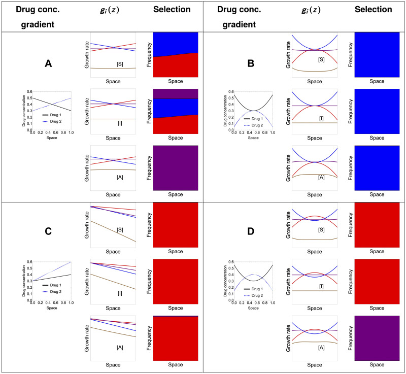
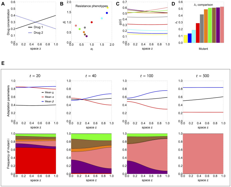
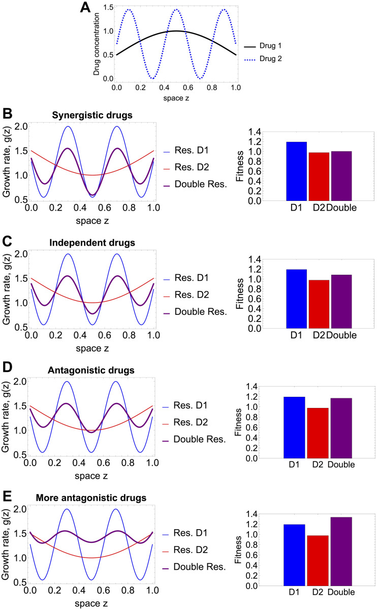
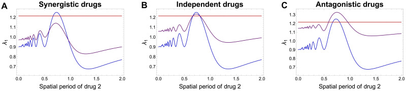
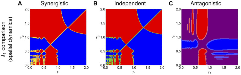
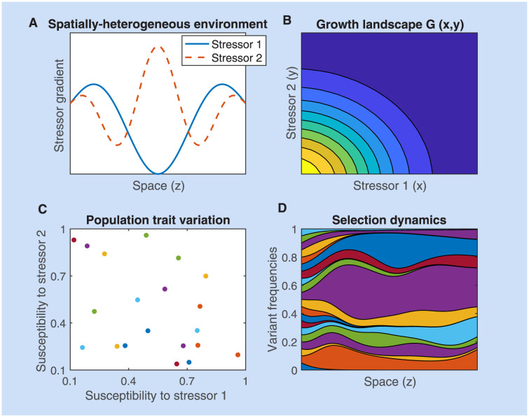
Multi-drug combinations to treat bacterial populations are at the forefront of approaches for infection control and prevention of antibiotic resistance. Although the evolution of antibiotic resistance has been theoretically studied with mathematical population dynamics models, extensions to spatial dynamics remain rare in the literature, including in particular spatial evolution of multi-drug resistance. In this study, we propose a reaction-diffusion system that describes the multi-drug evolution of bacteria based on a drug-concentration rescaling approach. We show how the resistance to drugs in space, and the consequent adaptation of growth rate, is governed by a Price equation with diffusion, integrating features of drug interactions and collateral resistances or sensitivities to the drugs. We study spatial versions of the model where the distribution of drugs is homogeneous across space, and where the drugs vary environmentally in a piecewise-constant, linear and nonlinear manner. Although in many evolution models, per capita growth rate is a natural surrogate for fitness, in spatially-extended, potentially heterogeneous habitats, fitness is an emergent property that potentially reflects additional complexities, from boundary conditions to the specific spatial variation of growth rates. Applying concepts from perturbation theory and reaction-diffusion equations, we propose an analytical metric for characterization of average mutant fitness in the spatial system based on the principal eigenvalue of our linear problem, λ1. This enables an accurate translation from drug spatial gradients and mutant antibiotic susceptibility traits to the relative advantage of each mutant across the environment. Our approach allows one to predict the precise outcomes of selection among mutants over space, ultimately from comparing their λ1 values, which encode a critical interplay between growth functions, movement traits, habitat size and boundary conditions. Such mathematical understanding opens new avenues for multi-drug therapeutic optimization.

Fig 1. Example of outcomes among two strains for constant g_i over space.

A. Competitive exclusion. In this example, strains start at uniform distribution over space, with g₁ > g₂, hence dynamics lead to a traveling wave solution for f₁(z, t) and f₂(z, t) with strain 1 traveling at faster speed and ultimately being the winner everywhere over long time. B. (Neutrally-stable) coexistence at 50:50 because the mutants start at equal total abundances and g₁ = g₂. C. (Neutrally-stable) coexistence different from 50:50 because mutants start at different total abundances and g₁ = g₂. D. (Neutrally-stable) coexistence different from 50:50 because mutants start at equal total abundances with g₁ = g₂, but their initial distribution over space favours one of them that starts at higher abundance in the center of the domain.

Fig 2. Coexistence example of 2 strains everywhere in space for space-dependent g_i(z) which are mutually symmetric about L/2.

A. In this case, one strain is better-adapted in the first half of the domain, the other strain is better-adapted in the second-half of the domain with the selective advantages exactly counterbalanced. B. For low diffusion, the two strains coexist such that each strain dominates in frequency in the part of the domain where it experiences a relatively higher growth rate, maintaining a high-degree of spatial segregation in the system. C. As diffusion increases, the coexistence frequencies become more similar and tend towards 1/2 in both halves of the domain. D. Eventually, for very high-diffusion, the growth variation starts to matter less and less, and the two strains tend to the same frequency everywhere, leading to a uniformly homogeneous spatial distribution of diversity over space.

Fig 3. Competitive exclusion everywhere in space, but the ultimately winning strain depends on parameters of g_i(z) variation.

A. In this piece-wise growth rate example, the g₁(z) and g₂(z) are such that the mean growth rates for both strains are the same $\overline{g_1}={\int }_0^1{g}_1\left(z\right)dz={\int }_0^1{g}_2\left(z\right)dz=\overline{g_2}$ for b = 1/2 and g_max = 0.5, g_min = 0.3. Yet, even with equal spatially-averaged growth rates, starting from equal initial distributions, the strain with the central advantage will be the winner. When b changes, the final winner is a result of b as well as (max(g) − min(g)) magnitude. B. In this example, the winner can be overturned by modulating the width of the interval where g₁(z) > g₂(z), while keeping the shape of the two functions. We assume the growth rates are non-monotonic functions of space, represented by a concave and a convex parabola with vertices near the middle of the domain:g₁(z) = m − σ(z − L/2)² + h and g₂(z) = m + 2σ(z − L/2)² with m = 0.3, σ = 0.4, D = 0.015 and h varied. The critical value of h for overturning the final outcome is h = 0.04. Mutant 1 loses if h < 0.04 but it wins if h > 0.04, when its fitness advantage in the center of the domain is sufficiently high to compensate for its disadvantage near the boundaries. This cannot be predicted with the mean growth rate difference $\overline{g_1}-\overline{g_2}$ but can be predicted with λ₁ difference for mutants 1 and 2. See also S1 Mathematica Notebook.

Fig 4. The basis for the atlas of multi-drug resistance evolution patterns over space.

A. The four canonical mutant types for resistance phenotypes to two drugs, distributed in the (α, β) space of rescaling parameters: blue—fully resistant to drug 1 and sensitive to drug 2; red—fully resistant to drug 2 and sensitive to drug 1; purple—intermediate resistance to both drugs; brown—wild-type, sensitive to both drugs. The 3 drug fitness landscapes used are: B. synergistic, C. independent and D. antagonistic, as specified in Eq 16 for q = 1. These drug landscapes will be used to give rise to g_i(z) = G(α_ix(z), β_iy(z)) as a function of two drug variation over space x(z) and y(z). The relative fitnesses of the strains are hence dependent both on drug variation over space and on the details of the underlying growth landscape G.

Fig 5. An atlas for 2-drug resistance evolution in space under spatial heterogeneity.

We consider only four available mutants each with different resistance phenotypes to two drugs, distributed in the (α, β) space of rescaling parameters: blue—fully resistant to drug 1 and sensitive to drug 2; red—fully resistant to drug 2 and sensitive to drug 1; purple—intermediate resistance to both drugs; brown—wild-type, sensitive to both drugs. We considered a diffusion coefficient of D = 0.01; the spatial equilibrium is obtained numerically by considering the system at t = 400. For all the simulations, we considered the same initial distributions with 99% wild type mutants and the remaining 1% distributed equally among the three resistant mutants. The initial distributions of each mutant were shaped as the function $\text{sin}\left(\frac{\pi z}{L}\right)$, so that the homogeneous Dirichlet boundary conditions were respected. The growth landscapes were as specified in Eq 16. The interaction strength is fixed at q = 1 both in the case of synergistic and antagonistic interaction. For more drug gradient scenarios, under a more complex drug interaction profile and two diffusion rates, see Supplementary Figs A-C in S1 Text.

Fig 6. Validating selection predictions based on λ₁ ranking among several competing mutants.

We illustrate a model simulation under the linear drug gradients in A, with 10 multi-drug resistant mutants varying in (α_i, β_i) traits (B), growing (g_i(z) in C) and spreading over space with diffusion coefficient D = 0.01. The λ₁ values (Eq 14) in D, match very well with the spatial selection dynamics observed numerically (E). Initial conditions (99% vs 1%: WT vs. equal division among all the mutants) were assumed equal for all strains, satisfying the boundary conditions n_i(z, 0)∼sin(πz).

Fig 7. Selection outcomes for periodic drug regimes leading to periodic growth rates over space.

A. The periodic variation of drug 1 and drug 2 over space, keeping the total amount of each drug equal. The periodic function parameters, under conservation of total drug, are: k₁ = A₁ = 0.5, T₁ = 2 and k₂ = A₂ = 0.72, T₂ = 0.4. Further we show mutant growth rates and selection outcome following the linear G function combinations in Eq 16 under: B. synergistic drug interactions (strength q = 0.5); C. independent drugs; D. antagonistic drug interactions (strength q = 0.5); E. even more antagonistic drugs (strength q = 1.5). The first column shows resulting growth rates g_i(z) for each mutant. The second column shows associated principal eigenvalues for each of the 3 mutants over space, computed as an indicator of overall fitness where D1 refers to the mutant resistant to drug 1, D2 the mutant resistant to drug 2 and Double, the mutant partially resistant to both drugs. Assumed diffusion coefficient is D = 0.01. (See also S4 Mathematica Notebook for this case).

Fig 8. Fitness ranking among 3 mutants for periodic drug regimes, as a function of spatial period of drug 2.

A. Synergistic drug interaction. B. Independent drug action C. Antagonistic drug interaction. The strength of interaction when assumed, was q = 0.5 and G(x, y) were specified as in Eq 16. The periodic variation of drug 1 x(z) was held fixed, while drug 2 concentration y(z) over space was varied by varying the period T₂. These parameters were fixed: k₁ = A₁ = 0.5, T₁ = 0.8 and k₂ = A₂ = 0.5 before normalization, which then leads to total conservation of drug 1 and drug 2, fixed amount = 1 for each spatial period of drug 2 T₂. Final fitnesses of the 3 mutants over space, computed on the basis of the principal eigenvalue. Assumed diffusion coefficient is D = 0.01. In blue: single-resistance to drug 1, in red: single-resistance to drug 2, in purple: double resistant mutant with intermediate resistance to each drug.

Fig 9. Drug-resistance selection outcomes for periodic 2 drugs as a function of their spatial periods T₁ and T₂.

A. Synergistic drugs. B. Independent drugs. C. Antagonistic drugs. Shaded blue region: single-resistance to drug 1 has higher fitness, shaded red region: single-resistance to drug 2 has higher fitness, shaded purple region: double resistant mutant with intermediate resistance to each drug has the higher fitness. The periodic variations of drug 1 and drug 2 over one-dimensional space z ∈ [0, 1] are constructed in such way as to keep the total amount of each drug equal to 1. The periodic function parameters are initially specified as: k₁ = A₁ = k₂ = A₂ for any combination of periods T₁ and T₂, and then immediately scaled by the integral of the periodic function over space, to obtain a total amount of drug equal to unity in each case. Assumed diffusion coefficient is D = 0.01. The growth functions of each mutant over space are obtained following Eqs. 16 together with the assumption that a mutant with traits (α_i, β_i) experiences the two drugs at concentrations α_ix and β_iy. The interaction strength is fixed at q = 0.5 both in the case of synergistic and antagonistic interaction. In the case of synergistic/antagonistic interaction, the effect is to decrease/increase the growth rate of bacteria relative to the simple additive effect of the two drugs. See Fig D (S1 Text) for the analogous figure under a more complex drug interaction function, highlighting the sensitivity to fitness landscape.

Model translation to environmental contexts beyond antibiotics.

A. Two arbitrary spatially-varying stressors (1 and 2). B. The growth landscape G(x, y) of the reference (WT) strain as a function of stressor concentrations forms the basis for building later the growth landscapes of different mutants. C. The primary dose-responses of stressor- to- growth phenotypic effect can be used to obtain (α_i, β_i) traits in the sub-populations of interest. D. These coefficients are then used to rescale G accordingly to obtain growth rates g_i(z) for all variants under various stressor concentrations. With these ingredients, the model can be applied to other ecological contexts.

References

1. Laxminarayan R, Duse A, Wattal C, Zaidi AK, Wertheim HF, Sumpradit N, et al.. Antibiotic resistance?the need for global solutions. The Lancet infectious diseases. 2013;13(12):1057–1098. doi: 10.1016/S1473-3099(13)70318-9 - DOI - PubMed
1. Cassini A, Högberg LD, Plachouras D, Quattrocchi A, Hoxha A, Simonsen GS, et al.. Attributable deaths and disability-adjusted life-years caused by infections with antibiotic-resistant bacteria in the EU and the European Economic Area in 2015: a population-level modelling analysis. The Lancet infectious diseases. 2019;19(1):56–66. doi: 10.1016/S1473-3099(18)30605-4 - DOI - PMC - PubMed
1. Marston HD, Dixon DM, Knisely JM, Palmore TN, Fauci AS. Antimicrobial resistance. Jama. 2016;316(11):1193–1204. doi: 10.1001/jama.2016.11764 - DOI - PubMed
1. Murray CJ, Ikuta KS, Sharara F, Swetschinski L, Aguilar GR, Gray A, et al.. Global burden of bacterial antimicrobial resistance in 2019: a systematic analysis. The Lancet. 2022;399(10325):629–655. doi: 10.1016/S0140-6736(21)02724-0 - DOI - PMC - PubMed
1. Beardmore RE, Pena-Miller R, Gori F, Iredell J. Antibiotic Cycling and Antibiotic Mixing: Which One Best Mitigates Antibiotic Resistance? Molecular Biology and Evolution. 2017;34(4):802–817. doi: 10.1093/molbev/msw292 - DOI - PMC - PubMed