Causal Cortical and Thalamic Connections in the Human Brain

Abstract

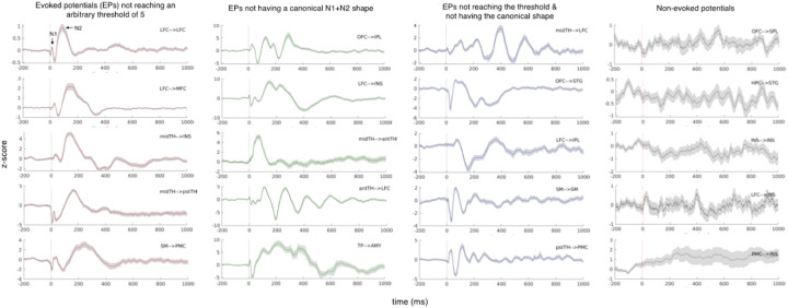
The brain's functional architecture is intricately shaped by causal connections between its cortical and subcortical structures. Here, we studied 27 participants with 4864 electrodes implanted across the anterior, mediodorsal, and pulvinar thalamic regions, and the cortex. Using data from electrical stimulation procedures and a data-driven approach informed by neurophysiological standards, we dissociated three unique spectral patterns generated by the perturbation of a given brain area. Among these, a novel waveform emerged, marked by delayed-onset slow oscillations in both ipsilateral and contralateral cortices following thalamic stimulations, suggesting a mechanism by which a thalamic site can influence bilateral cortical activity. Moreover, cortical stimulations evoked earlier signals in the thalamus than in other connected cortical areas suggesting that the thalamus receives a copy of signals before they are exchanged across the cortex. Our causal connectivity data can be used to inform biologically-inspired computational models of the functional architecture of the brain.

Figure 1. Electrophysiological responses (local field potential) evoked by the stimulation of a given brain area are complex and variable.

Here we show randomly selected examples of the complex waveforms generated by electrical stimulation. A large portion of evoked responses either does not reach an arbitrary threshold, e.g., z-score = 5 that is usually used in the literature (first column, with five separate examples) or does not conform to a typical shape of evoked responses with an N1 and N2 components (second column) or neither have a large amplitude nor a canonical N1 and N2 shape (third column). By using univariate measures, one will only map a fraction of true connections in the brain. Plotted signals are the evoked responses stimulated and recorded from a pair of bipolar sites (i.e., from one stimulation bipolar site to one recording bipolar site), of which the anatomical information is provided in the upper corner. The central line is the trials-averaged signal, baseline-corrected and z-scored, while the shaded area depicts the standard error over the 45 trials.

Figure 2. Illustration of data processing pipeline.

(a) Electrode coverage at the group level. The electrode localization was manually labelled by the experienced neurologist on the team, based on each subject’s brain morphology in their own high-resolution T1 scan (L: left, R: right, ant: anterior, pst: posterior, PMC: posteromedial cortex, SM: sensorimotor, SPL: superior parietal lobule, ACC: anterior cingulate cortex, CLT: claustrum, TH: thalamus, IPL: inferior parietal lobule, MFC: medial frontal cortex, OFC: orbital frontal cortex, STG: superior temporal gyrus, LFC: lateral frontal cortex, INS: insula, FG: fusiform gyrus, HPC: hippocampus, MTG: middle temporal gyrus, PHG: parahippocampal gyrus, AMY: amygdala, TP: temporal pole, MCC: midcingulate cortex, ITG: inferior temporal gyrus). For visualization purposes, each subject’s brain images were normalized to a standard brain surface space (FS_LR: https://osf.io/k89fh/wiki/Surface/) with FreeSurfer (https://surfer.nmr.mgh.harvard.edu/) and Connectome-Workbench (https://www.humanconnectome.org/software/connectome-workbench), and their electrodes were projected to the standard surface (sites out of grey matter are excluded). (b) The localization of electrodes in the thalamus, divided into three thalamic divisions: anterior (purple), mid (blue), and posterior (green) subregions of the thalamus, (c) Roadmap of data analysis. (d)Dimensionality reduction of the evoked spectral information of all pair-wise evoked potentials in the activated cluster (i.e., pairs with underlying connections). The spectral information is the concatenated power and inter-trial phase coherence (ITPC) spectrograms of the evoked potentials, which are down-sampled to balance the number of datapoints for earlier and later neural responses (see Methods). While this figure is not intended to show distinct clusters, we have colored the dots (a posteriori) to illustrate that data from ipsilateral thalamic stimulations (red dots) are already distinguishable upon a visual inspection. Notably, the color patterns follow different stimulation sites but for recording sites (also see SI Fig. S3 a,c,d). They are not biased by specific subjects (SI Fig. S4). (e)Neural feature encoding involved two main steps: UMAP supervised learning and cluster-based permutation testing. The input data was the evoked power and ITPC spectrograms of the group-level whole-brain evoked potentials, while the dependent variable (i.e., the labels) were the ipsilateral cortical (COR-ipsi), ipsilateral thalamic (THAL-ipsi), contralateral cortical (COR-contr), and contralateral thalamic (THAL-contr) pairs. The algorithm successfully characterized these evoked spectrograms into the four categories. HDBscan was used to formally define the clusters in the embedding space, dissociating them from noisy channels. Original spectrograms of the pairs clustered in the four categories were then used to perform cluster-based permutation testing, by which we identified three time-frequency clusters within the spectrograms that were specific to each category (i.e., Neural Feature). Before statistical testing, the evoked power spectrograms of the four stimulation sites already show distinct features that can be distinguishable by visual inspection alone (marked by white circles and numbered).

Figure 3. Spectrograms of stimulation-evoked power within and between anatomical categories

(COR: cortex, THAL: thalamus, ipsi: ipsilateral, contr: contralateral, à: causal influence direction). Highlighted contours on the spectrograms indicate significant clusters (n-permutation = 5000, initial duster forming threshold = 6 t-scores, P_cluster < 0.01). Dashed lines on the spectrograms denotes the segments of conventional frequency bands: [0.5, 5] Hz (delta), [5, 8] Hz (theta), [8, 15] Hz (alpha), [15, 30] Hz (beta) [30, 70] Hz (gamma) and > 70 Hz (high). Same tests were conducted on ITPC spectrograms, which generated similar results Fig. S6) The frequency axis is in a logarithmic (log) scale. The time axis is unevenly sampled to balance the varied lengths for different clusters (see Method “training data preparation”), (a) Thalamic and cortical evoked spectrograms and significant clusters in either ipsilateral or contralateral hemispheres. Significance testing conducted using within-subject one-sample t-test (in a mixed-model design): individual-level t-statistics input into a group-level significance testing. The color bars show group-level t-scores. The color bars show group-level t-scores; significant clusters of the one-sided test is marked by white contours. These spectrograms, without significant markers, have also been used in Figure 2e for illustration, (b) Thalamic vs. cortical evoked spectrogram comparison using within-subject two-sample t-test (two-tailed) on the power spectrograms, significance inference performed with cluster-based permutation testing. Yellow and blue contours respectively highlight significant clusters of the contrast indicated on the subtitle and its reversed contrast. Acronym example “THAL-ipsi” on the subtitle means ipsilateral pairs stimulating from thalamus, (c) Intra-thalamic, thalamocortical, corticothalamic and cortico-cortical evoked spectrogram comparisons. Acronym example “THAL-ipsi” means ipsilateral pairs stimulating from the thalamus. Significant clusters of the one-sided tests are marked by white contours. For THAL->THAL (contra) connections, no significant cluster was generated here as there were not enough subjects (n<10) to provide sufficient statistical power for the mixed-model testing. However, a significance test can be done at the level of electrode contacts (i.e., without considering the grouping factor of “subject”). This alternative analysis showed a consistent pattern with the subject-averaged spectrogram, and resulted in two significant clusters, one in the gamma band before 60ms, another in the alpha/theta band around 100–275 ms (Fig. S8). Acronym example “THAL-THAL (ipsi)” on the subtitle means ipsilateral pairs stimulating from the thalamus and recording from the thalamus.

Figure 4. Electrophysiological neural features indicating different types of connectivity and illustration of the decoding process.

(a) Neural features specified by the spectra-temporal information. The time windows of the neural features are circumscribed by the significant clusters distinct among conditions from the previous cluster-based permutation testing. The time-frequency relationships in the three features are represented by the group-averaged spectrograms of the COR-ipsi, COR-contr and THAL-contr stimulations, as these three categories show clearest and non-overlapped significant clusters at the group level. The frequency axis is in log-scale. The time axis is in a natural scale with even samples, different from the time axis in Figure 3. The values of power and ITPC spectrograms are transformed (logarithmized and square-rooted, respectively) to approximate Gaussian distributions, and then zscored (in both time and frequency directions) to be comparable among connections. Line plots to the right of the spectrograms show the (normalized and log-scaled) spectral density of the power and ITPC during the significant time window, with colored lines for all the time points, and black for the time average. Since the evoked spectrograms were baseline-corrected, depicted curves can be seen as the “bumps” on top of the 1/f background noise. Group-averaged evoked potentials at the temporal domain corresponding to each category of the spectrograms are shown below, (b) Cross-correlation with a sliding window approach. To reveal the presence of each feature in individual connections, the feature information (i.e. the short-lasting spectral information characterized by the power and ITPC in the time-frequency window) is correlated to the spectrograms with Person-correlation r. To examine this correspondence at every time point (sampling rate is 200 per second), an over-lapping sliding window approach is used, whereby the “transient” time-frequency information at each time point is examined while the examining window is sliding over the spectrograms. This generates the dynamic appearance of the feature presence over time. The line plot in the middle is an example case randomly selected form the THAL-contr instances. Every point on the curve, with a specific time in x-axis and similarity measure in y-axis, indicates how similar the current spectral information (power and ITPC sustaining in certain amount of time) matches the neural feature in concern. The maximum r (r*) and the time to r* (latency) was taken as indices of feature representation and analyzed in the subsequent analyses. The heatmap to the right shows the correlation between all the THAL-contr instances and the Feature 3 (F3). An overview of feature presence in all categories of all features is presented in Fig. S.9.

Figure 5. The timing of feature presence (i.e., latency of maximum representation of the feature).

(a) The top panel shows the distribution of the latencies of F1 presence in all types of connections. F1 is identified in individual instances by finding the peaks of the feature curve. Included in the distribution are connections with strong F1 representation (r* > 0.4) which falls in a sensible latency range of (10, 70) ms, based on our results. Density distributions for thalamocortical connections are filled red, corticothalamic connections are filled blue, and thalamo-thalamic/cortico-cortical connections are filled grey. Colors for contralateral connections are lighter than those for ipsilateral connections. The middle panel is a cartoon showing the median latency of the feature presence among the aforementioned connections. The lower panel depicts within-subject post-hoc comparisons (adjusted for individual and regional differences) between the categories that showed evident differences in the latency distributions. Each colored dot marks the mean latency of all the connections from one subject. The black bar through the dot marks the range of ± one standard error of the within-subject data. Grey lines across groups show the within-subject comparisons. All tests were corrected for multiple comparisons. The full list of post-hoc comparisons is presented in SI Table S9. (b) and (c) shows F2 and F3 results with same visualization schemes. The criteria for data going into the F2 distributions are r* > 0.4 and latency in (70, 165) ms. The criteria for the F3 distributions are r* > 0.5 and latency in (200, 400) ms. As there were much fewer contralateral thalamocortical connections with F1 and F2, the data for these two features showed large variabilities.

Figure 6. The anatomical landscapes of feature presence.

(a) Early F1 connectivity matrices for bilateral cortical and thalamic subregions (l: left, r: right, ant: anterior, pst: posterior, PMC: posteromedial cortex, SM: sensorimotor, SPL: superior parietal lobule, ACC: anterior cingulate cortex, CLT: claustrum, TH: thalamus, IPL: inferior parietal lobule, MFC: medial frontal cortex, OFC: orbital frontal cortex, STG: superior temporal gyrus, LFC: lateral frontal cortex, INS: insula, FG: fusiform gyrus, HPC: hippocampus, MTG: middle temporal gyrus, PHG: parahippocampal gyrus, AMY: amygdala, TP: temporal pole, MCC: midcingulate cortex, ITG: inferior temporal gyrus); The anatomical localization of all electrode contacts was visually inspected and labeled by an experienced neuroanatomist using the position of the electrodes in the individual subject’s native brain space. Each entry of the matrix has a row and column identity corresponding to site of stimulation and recording, respectively, and its value indicates the feature representation (R) for the corresponding feature. Specifically, R = r⁻, was averaged across connections where the feature was present. Feature presence was binarized with a threshold of r*>0.4 for F1,2 and r*>0.5 for F3. Arbitrary thresholding was applied only for visualization purposes; un-thresholded matrices are presented in the SI Fig. S10. From the matrix, three entries were randomly chosen, with graded R values from low to high, to demonstrate their associated evoked responses in the time domain. For plotting the evoked responses, the black line is the site-averaged signal across the evoked potentials stimulated/recorded in the same anatomical regions – it is a group-level average which may involve different subjects whose stimulated/recording sites are in the same brain region. The grey-shaded area around the line is the standard error over sites. (b) Delayed F3 connectivity matrices for bilateral cortical and thalamic subregions with the same visualization scheme as aforementioned. (c) and (e) show brain heatmaps of the contrasted feature representation among the thalamic divisions (antTH vs. pstTH, midth vs. pstTH, midTH vs. pstTH), respectively for the thalamic inflow (i.e., recording in the thalamus) and outflow (i.e., stimulation in the thalamus) pathways. All values were projected to one hemisphere for compact visualization. FS_LR brain surface space (with symmetric left and right hemisphere) is used to minimize the visualizing bias caused by interhemispheric anatomical differences (https://osf.io/k89fh/wiki/Surface/). Grey dots on the brain surface indicate electrode coverage, and the color radius around the dots indicate local R values of the given contact. Due to sparse recording, the color is also projected to the brain surface with a Gaussian function over distance from the source, to approximate a whole-brain level estimation. Coloring intensity on the brain surface has been adjusted for regional density of electrode coverage. The presented brain heatmaps are not thresholded; formal statistical testing results and model details can be found in Table S2–5.

Figure 7.. Late thalamocortical compared with early corticothalamic connections.

Causal connectivity matrices are adapted from Figure 4 where the details can be found. These are shown again to indicate the data used for the respective brain heatmap plots, (a) The brain heatmap shows the comparison between F1-outflow vs. F3-outflow representations measured in each recording site across the brain due to stimulation of the anterior, mid-, and posterior thalamic subregions corresponding to anterior, mediodorsal, and pulvinar nuclei of the thalamus. Since we did not have hypotheses about hemispheric lateralization of connectivity profiles, we projected all electrodes onto one hemisphere for compact visualization. FS_LR brain surface space (with symmetric left and right hemispheres) was used to minimize the visualization bias caused by interhemispheric anatomical differences (https://osf.io/k89fh/wiki/Surface/). The color bar shows normalized feature representation: $\overline{zscore(r*)}$ averaged across the stimulation sites Before averaging, the r* values of all the thalamic connectivity with the same feature type were z-scored, i.e., zscore(r*\F1,,THAL_{inflow&outflow}), zscore(r*\F3,THAL_{inflow&outflow}), in order to make the feature representations between pathways/feature types comparable. The distributions of these normalized z-scores are presented below the connectivity matrices. The positive (brown) patches represent contrasted z-scores of F3-outflow (out3) being greater than F1-outflow (out1), while blue patches represent brain regions where F1 outflow (out1) is greater than F3 outflow (out3) representation To avoid negative values being subtracted to become a positive value, negative z-scores were zeroed before being contrasted Grey dots on the brain surface indicate electrode coverage, (b) Same visualization scheme for the comparison of F3-outflow vs. F1-inflow pathways of the thalamus. The presented brain heatmaps are not thresholded; formal statistical testing results are presented in supplementary Table S6–7

References

1. Sporns O., Chialvo D. R., Kaiser M. & Hilgetag C. C. Organization, development and function of complex brain networks. Trends Cogn. Sci. 8, 418–425 (2004). - PubMed
1. Shine J. M., Lewis L. D., Garrett D. D. & Hwang K. The impact of the human thalamus on brain-wide information processing. Nature reviews. Neuroscience (2023). 10.1038/s41583-023-00701-0 - DOI - PMC - PubMed
1. Matsumoto R. et al. Functional connectivity in the human language system: a cortico-cortical evoked potential study. Brain 127, 2316–2330 (2004). - PubMed
1. Matsumoto R. et al. Functional connectivity in human cortical motor system: a cortico-cortical evoked potential study. Brain 130, 181–197 (2007). - PubMed
1. Wu T. Q. et al. Multisite thalamic recordings to characterize seizure propagation in the human brain. Brain 146, 2792–2802 (2023). 10.1093/brain/awad121 - DOI - PMC - PubMed
Publication types
LinkOut - more resources