A virtual rodent predicts the structure of neural activity across behaviours

Abstract

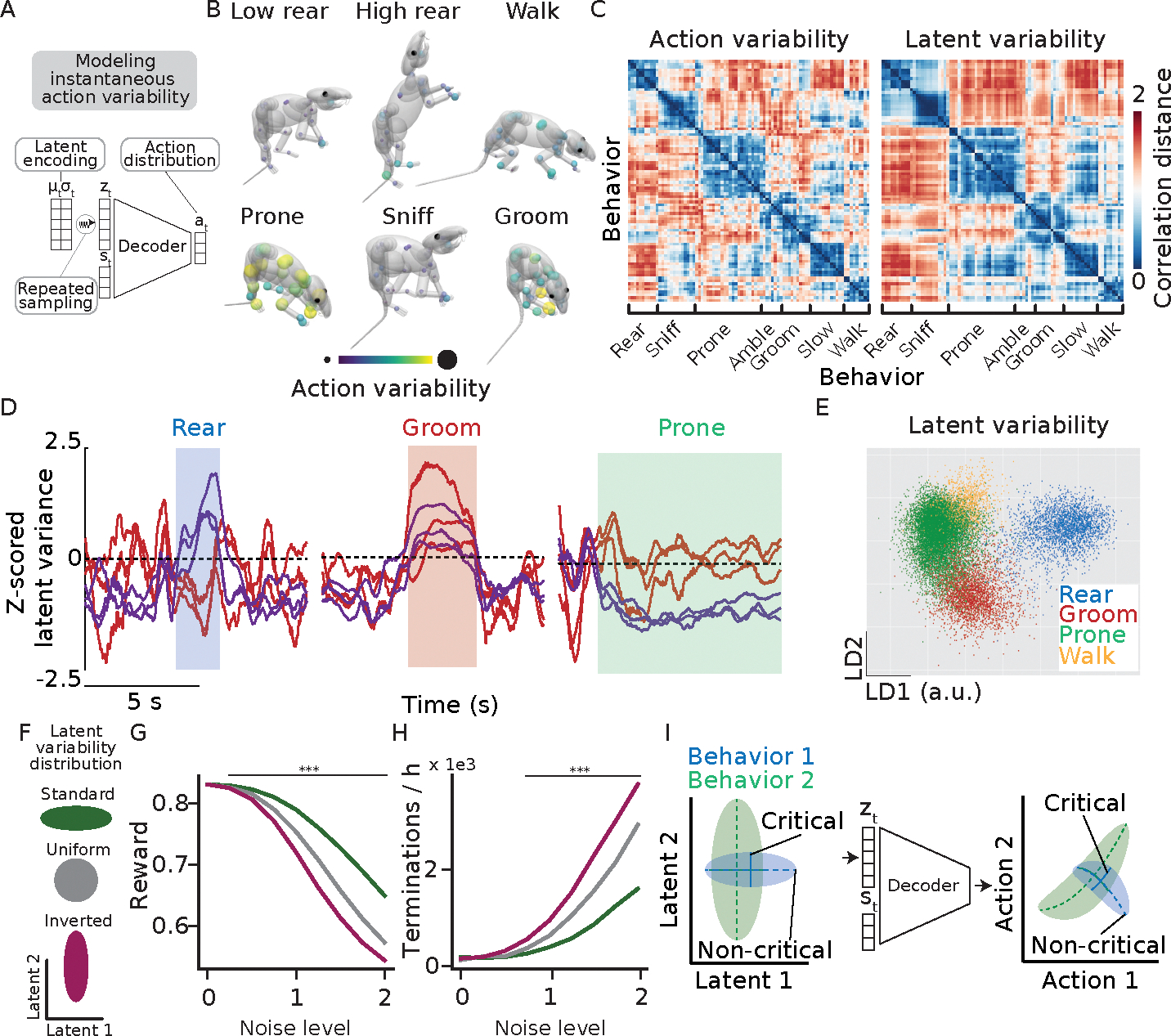
Animals have exquisite control of their bodies, allowing them to perform a diverse range of behaviours. How such control is implemented by the brain, however, remains unclear. Advancing our understanding requires models that can relate principles of control to the structure of neural activity in behaving animals. Here, to facilitate this, we built a 'virtual rodent', in which an artificial neural network actuates a biomechanically realistic model of the rat¹ in a physics simulator². We used deep reinforcement learning^3-5 to train the virtual agent to imitate the behaviour of freely moving rats, thus allowing us to compare neural activity recorded in real rats to the network activity of a virtual rodent mimicking their behaviour. We found that neural activity in the sensorimotor striatum and motor cortex was better predicted by the virtual rodent's network activity than by any features of the real rat's movements, consistent with both regions implementing inverse dynamics⁶. Furthermore, the network's latent variability predicted the structure of neural variability across behaviours and afforded robustness in a way consistent with the minimal intervention principle of optimal feedback control⁷. These results demonstrate how physical simulation of biomechanically realistic virtual animals can help interpret the structure of neural activity across behaviour and relate it to theoretical principles of motor control.

Extended Data Figure 1.. Recording neural activity in freely behaving rats.

A) Schematic of custom 128-channel tetrode drive. B) Tetrodes record electrical events of several putative neurons from the DLS or MC. Shown are recordings from a tetrode in DLS. C) Individual putative cells are extracted based on their unique spike waveforms using a custom spike-sorting software, FAST. D) Tetrodes allows for the recording of hundreds of putative single units simultaneously. E-F) Representative examples of Nissl-stained brain slices from animals with electrophysiological implants in DLS and MC. Red ellipses indicate the lesions remaining from the tetrode implants. G) Dorsal view denoting the position of implants for DLS and MC. The position of the implant with the dashed circle could not be verified with histology as the recording headstage was dislodged prior to electric lesion. The position was instead estimated using scarring at the cortical surface and the recorded depth of implantation. The other implants were verified with electric lesions or scarring from the implant tip. H) Coronal plane indicating the location of implants in the DLS across 3 animals. I) Coronal plane indicating the location of implants in MC across 3 animals.

Extended Data Figure 2.. High fidelity 3D pose estimation and skeletal registration.

A) In DANNCE, a 3D U-Net processes multi-view images to estimate the positions of 23 3D keypoints across the rat’s body. B) DANNCE keypoint estimates show high concordance with manual annotations, deviating from manual labels to a similar degree as repeated manual annotations of the same testing frames. C) Visualization of median DANNCE keypoint discrepancy relative to manual annotation. Gray circles indicate the bounds of the sphere with radius equal to the median keypoint discrepancy for each keypoint. D) Schematic depicting the relevant variables in STAC. STAC operates by jointly optimizing a set of offsets relating the skeletal model to different keypoints and the pose of the model in each frame. E) STAC registration is highly accurate across body parts and F) across different behaviors. For all boxplots in this figure, colored lines indicate the median, boxes indicate the interquartile range, and whiskers indicate the 10th and 90th percentiles.

Extended Data Figure 3.. Comparing imitation performance for held-out data across different classes of control networks.

A) The proportion of episodes exceeding a given duration for the four classes of controllers. Results for each class are averaged across models with all KL regularization coefficients for that class. B) Violin plots showing the distribution of rewards by each model class on the held-out testing set. Models with LSTM decoders outperform other classes. C) Average reward as a function of the center of mass speed for each class of controller. LSTM models outperform other model classes across all speeds, but especially at slow speeds. D) Box plots denoting the distribution of rewards for each model class as a function of behavior category. LSTM models outperform other classes across all behavior, but especially those with slow center of mass speed. White lines indicate the median, box limits indicate the interquartile range, box whiskers indicate the 10th and 90th percentiles. E) The proportion of episodes exceeding a given duration for models with LSTM decoders across all KL regularization coefficients. Models with higher KL regularization are generally less robust than those with lower KL regularization, consistent with an increase in latent noise. F) Violin plots denoting the distribution of rewards on held-out natural behavior for each model as a function of KL regularization. Increasing the KL regularization coefficient marginally decreases the reward distribution of the models. White lines indicate the median. G) We trained five models with different reference window lengths using an LSTM decoder with a KL regularization of 1e-4. Violin plots denote the distribution of rewards on held-out natural behavior for each model. Models with reference windows of length 5 or shorter exhibit comparable performance, while a reference window of 10 exhibits poorer performance. Gray lines indicate the quartiles. H) The proportion of episodes exceeding a given duration. Models with longer reference window length are generally more robust than those with shorter reference window lengths, with the most robust model being that with a reference window length of 5. Shaded regions indicate the standard error of the mean over sessions. I) The distribution of joint angles during imitation closely match those of STAC-registered skeletal models during imitation. Data is from a model with an LSTM decoder and a KL regularization of 1e-4. Box centers indicate the median, box limits indicate the interquartile range, box whiskers indicate the maximum or minimum values up to 1.5 times the interquartile range from the box limits.

Extended Data Figure 4.. Neurons in the DLS and MC encode posture across many body parts to a degree consistent with previous reports during unrestrained behavior.

A, C) Proportion of neurons in DLS and MC best predicted by each feature class. B, D) Violin plots showing the distribution of cross-validated log-likelihood ratios (CV-LLR) of GLMs trained to predict spike counts using different feature classes. E, F) Box plots showing the distribution of deviance-ratio pseudo r-squared values of GLMs trained to predict spike counts using different feature classes. White lines indicate the median, boxes indicate the interquartile range, and whiskers indicate the 10th and 90th percentiles. G, H) Empirical cumulative distribution functions denoting the proportion of neurons in DLS and MC with peak GLM predictivity below a given pseudo r-squared value. The distributions resemble previous reports in rats during spontaneous behavior .

Extended Data Figure 5.. Encoding properties are similar across striatal cell types.

A-C) Proportion of neurons in DLS and MC best predicted by each feature class for each cell type. D-F) Box plots showing the distribution of cross-validated log-likelihood ratios relative to a mean firing rate model for GLMs trained to predict spike counts using different feature classes. White lines indicate the median, boxes indicate the interquartile range, and whiskers indicate the 10th and 90th percentiles. G-H) Comparison of the best computational feature derived from the network and representational feature GLM CV-LLRs for each neuron. GLMs based on the inverse dynamics models (computational features) outperform those based on representational features for the majority of classified neurons for all cell types (p < .001, permutation test).

Extended Data Figure 6.. Neurons in the DLS and MC encode future movement during natural behavior.

We trained GLMs to predict neural activity from measurable features of movement and from features of the ANN controllers while introducing time lags ranging from −1000 ms to 300 ms between neural activity and the features. A) Histograms depicting the distribution of time lags for maximally predictive GLMs when using joint angle predictors. Time lags less than zero correspond to neurons whose future movements better predict neural activity (premotor), while time lags greater than zero correspond to neurons whose past movements best predict neural activity (postmotor). B) CVLLR relative to models trained with a time lag of 0 ms averaged across neurons. Shaded regions indicate the standard error of the mean. The peak average CVLLR occurs at −200 ms for all cell types. C, D) Same as A-B, except using features from the inverse dynamics model (LSTM hidden layer 1) as GLM predictors for a model with an LSTM decoder and a KL regularization of 1e-4. Peak predictivity occurs closer to a time lag of zero, consistent with the network’s representation of desired future state and inverse dynamics. E,F) Same as A-B for neurons in MC. G, H) Same as C-D for neurons in MC.

Extended Data Figure 7.. Comparing imitation performance and neural predictivity of models trained to control bodies of different masses.

A) We trained five models with an LSTM decoder and a KL regularization of 1e-4 to control bodies of different masses. Violin plots denote the distribution of rewards on held-out natural behavior for each model. Several models controlling bodies with masses other than the standard mass exhibited reduced performance. White lines indicate medians. B) The proportion of episodes exceeding a given duration. Shaded regions indicate S.E.M across individuals. C-D) Box plots depicting the distribution of cross-validated log-likelihood ratios across neurons of GLMs trained to predict neural activity from network features. The CVLLR for each neuron is expressed relative to the likelihood of a GLM trained to predict neural activity using network features from the standard mass model. Values greater than zero imply a model more predictive of neural activity than those derived from the standard mass model, and vice versa. White lines indicate the median, box limits indicate the quartiles, whiskers indicate the 10th and 90th percentiles. Stars indicate that a greater proportion of neurons are better predicted by GLMs trained using features from the standard mass model than from the alternative mass model (Bonferroni corrected, α = .05, permutation test). E-F) Average WUC similarity between RDMs derived from network layers and neural activity in DLS or MC. Error bars indicate S.E.M across individuals. Arrows indicate significantly different similarity distributions across animals (Benjamini-Hochberg corrected, false discovery rate α = .05, one-sided t-test).

Extended Data Figure 8.. Comparing imitation performance and neural predictivity of models trained to control bodies of the same total mass with different head masses.

A) We trained five models with an LSTM decoder and a KL regularization of 1e-4 to control bodies of the same total mass with different relative masses between the head and the rest of the body. Violin plots denote the distribution of rewards on held-out natural behavior for each model. Several models controlling bodies with masses other than the standard mass exhibited reduced performance. White lines indicate medians. B) The proportion of episodes exceeding a given duration. Shaded regions indicate S.E.M across individuals. C-D) Box plots depicting the distribution of cross-validated log-likelihood ratios across neurons of GLMs trained to predict neural activity from network features. The CVLLR for each neuron is expressed relative to the likelihood of a GLM trained to predict neural activity using network features from the standard mass model. Values greater than zero imply a model more predictive of neural activity than those derived from the standard mass model, and vice versa. White lines indicate the median, box limits indicate the quartiles, whiskers indicate the 10th and 90th percentiles. Stars indicate that a greater proportion of neurons are better predicted by GLMs trained using features from the standard mass model than from the alternative mass model (Bonferroni corrected, α = .05, permutation test). E-F) Average WUC similarity between RDMs derived from network layers and neural activity in DLS or MC. Error bars indicate S.E.M across individuals. Arrows indicate significantly different similarity distributions across animals (Benjamini-Hochberg corrected, false discovery rate α = .05, one-sided t-test).

Extended Data Figure 9.. The representational structures of DLS and MC resemble an inverse model more than alternative control models.

A) To compare the representational structure of neural activity in DLS and MC across different candidate computational models we used B) rollouts from an inverse model to collect state-action pairs to train C) forward and sequential models with supervised learning. D-F) Across-subject representational similarity between control models and neural activity. The latent representation of an inverse model more closely resembles the structure of neural activity in DLS and MC than the latent representation of forward or sequential models. G-I) The latent variability of an inverse model better predicts the structure of neural variability than representational models. Error bars indicate S.E.M. Icicles and dew drops indicate significant differences from the noise ceiling and zero (Bonferroni corrected, α = .05, one-sided t-test). Gray bars indicate the estimated noise ceiling of the true model. Arrows indicate significant differences between features (Benjamini-Hochberg corrected, false discovery rate α = .05, one-sided t-test). Points indicate individual animals.

Extended Data Figure 10.. Inverse dynamics models predict putative single-unit neural activity better than alternative control models and feedback.

A-B) Box plots showing the distribution of cross-validated log-likelihood ratios (CV-LLR) relative to mean firing-rate models of GLMs trained to predict spike counts using different feature classes. White lines indicate the median, boxes indicate the interquartile range, and whiskers indicate the 10th and 90th percentiles.

Figure 1.. Comparing biological and artificial control across the behavioral repertoire with MIMIC.

A) To compare neural activity in behaving animals to computational functions in control, we trained ANNs actuating a biomechanical model of the rat to imitate the behavior of real rats. B) (Top) Representational approaches in neuroscience interpret neural activity in relation to measurable features of movement. Computational approaches, in contrast, can relate neural activity to specific control functions, such as internal models. C-F) The MIMIC pipeline. C) (Left) Schematic of experimental apparatus for behavioral and electrophysiological recording. A tetrode array recorded electrical activity of neurons in DLS or MC. (Right) Example images taken during a walking sequence. D) (Left) Schematic of the DANNCE pose estimation pipeline. Multi-view images were processed by a U-net to produce keypoint estimates. (Right) Walking sequence with overlaid keypoint estimates. E) (Left) We registered a skeletal model of the rat to the keypoints in each frame using STAC. (Right) Walking sequence with overlaid skeletal registration. F) We trained an ANN to actuate the biomechanical model in MuJoCo to imitate the reference trajectories. (Right) Walking sequence simulated in MuJoCo.

Figure 2.. Training artificial agents to imitate rat behavior with MIMIC.

A) We train a virtual rodent to imitate the 3D whole-body movements of real rats in MuJoCo with deep reinforcement learning (see methods). All networks implement an inverse dynamics model which produces the actions required to realize a reference trajectory given the current state. All simulated data in this figure are derived from models with LSTM decoders. B) (Left) Keypoint trajectories of the real rat and (Right) model-derived keypoint trajectories of the virtual rat imitating the real rat’s behavior (Top, anterior-posterior axis; Bottom, height from the floor). C) Example sequences of a rat performing different behaviors. Overlays rendered in MuJoCo depict the imitated movements. D) Imitation on held-out data is accurate for all body parts and E) across different behaviors. The total error is the average Euclidean distance between the model and anatomical keypoints, while the pose error indicates the Euclidean distance up to a Procrustes transformation without scaling. Box centers indicate median, box limits indicate interquartile range, box whiskers indicate the maximum or minimum values up to 1.5 times the interquartile range from the box limits. Panels B-E feature data from a model with a recurrent decoder and a KL regularization of 1e-4. F) Accumulation of error as a function of time from episode initiation. Deviations from the reference trajectory accumulate over time, with drift in the position of the center of mass accounting for much of the total error. G) The proportion of episodes exceeding a given duration. Shaded regions indicate the standard error of the mean across all models with LSTM decoders. Panels D-G include data from 28 3-hour sessions, with 4 sessions drawn from each of 7 animals.

Figure 3.. Neural activity in DLS and MC is best predicted by an inverse dynamics model.

A) MIMIC enables comparisons of neural activity to measurable features of behavior and ANN controller activations across a diverse range of behaviors. (Top) Aligned keypoint trajectories and spike rasters for DLS neurons over a fifty-second clip of held-out behavior. (Bottom) Z-scored activations of the artificial neurons comprising the model’s action layer, latent mean, and LSTM cell layer 1 when imitating the same clip. The depicted network features an LSTM decoder and a KL regularization coefficient of 1e-4. B) Proportion of neurons in DLS and MC best predicted by each feature class. C) Box plots showing the distribution of cross-validated log-likelihood ratios (CV-LLR) of GLMs trained to predict spike counts using different feature classes relative to mean firing-rate models. Data includes neurons significantly predicted by each GLM (Benjamini-Hochberg corrected Wilcoxon signed-rank test, α = .05) from a total of N=732 neurons in DLS and 769 neurons in MC. White lines indicate the median, boxes the interquartile range, and whiskers the 10th and 90th percentiles. D) Comparing predictions from the best computational and representational features for each neuron. GLMs based on the inverse dynamics models outperform those based on representational features for the majority of classified neurons in both DLS and MC (p < .001, one-sided permutation test).

Figure 4.. The representational structure of neural populations in DLS and MC across behaviors resembles that of an inverse model.

A) Average normalized firing rate for single units in DLS and MC as a function of behavior. B) Average representational dissimilarity matrices (RDMs) for neural activity in DLS and MC, and the average of layers in the encoder and decoder. Row and column indices are equal across RDMs and sorted via hierarchical clustering on the average neural activity RDM across all animals. C-E) Across-subject average of whitened-unbiased cosine (WUC) similarity between RDMs of different computational and representational models and neural activity. Layers of the inverse dynamics model predict the dissimilarity structure of neural activity in DLS and MC better than representational models. Error bars indicate S.E.M. Icicles and dew drops indicate significant differences from the noise ceiling and zero (Bonferroni corrected, α = .05, one-sided t-test). Gray bars indicate the estimated noise ceiling of the true model. Open circles indicate the comparison model, downward ticks on the wings extending from the comparison model indicate significant differences between models (Benjamini-Hochberg corrected, false discovery rate α = .05, one-sided t-test). Points indicate individual animals (N=3 individuals in C and D, N=6 individuals in E). F) Comparing average imitation reward and the mean WUC similarity with DLS or MC neural activity on held-out data for all networks. The average WUC similarity is the average similarity of all network layers relative to neural activity for a given network. Each point denotes a single network across all animals for a given brain region. G) Comparison of average WUC similarity and the average episode length for all networks. H, I) Same as F-G, except each point denotes a single network-animal pair.

Figure 5.. Stochastic controllers regulate motor variability as a function of behavior by changing latent variability.

A) We estimate instantaneous action variability as the standard deviation of the set of actions obtained by resampling the latent space 50 times at every step. To avoid long-term temporal dependencies, simulations in this figure use a torque-actuated controller with a multi-layer perceptron decoder and a KL regularization coefficient of 1e-3. B) Action variability differs as a function of behavior (p < .001, one-sided permutation test; see methods). Each sphere corresponds to a single actuator; its color and size indicate its normalized action variability during the designated behavior. C) RDMs of action variability and latent variability across behaviors. D) Trajectories of six latent dimensions along which variability was differentially regulated across behavior. E) Scatter plot depicting the latent variability at single time points plotted on the first two linear discriminants for three behavioral categories. The population latent variability discriminates behaviors (p < .001, one-sided permutation test; see methods). F) Schematic depicting changes to the structure of latent variability (see text). G) The deviations from normal variability structure reduce the model’s robustness to noise (p < .001, one-sided Welch’s t-test) H) and termination rate (p < .001, one-sided Chi-squared test). Lines indicate significant differences between conditions. I) (Schematic) The latent variability is differentially shaped as a function of behavior to structure action variability in accordance with the minimal intervention principle.

References

1. Merel J et al. Deep neuroethology of a virtual rodent. in Eighth International Conference on Learning Representations (2020).
1. Todorov E, Erez T & Tassa Y MuJoCo: A physics engine for model-based control. in 2012 IEEE/RSJ International Conference on Intelligent Robots and Systems 5026–5033 (ieeexplore.ieee.org, 2012).
1. Hasenclever L, Pardo F, Hadsell R, Heess N & Merel J CoMic: Complementary Task Learning & Mimicry for Reusable Skills. 119, 4105–4115 (13–18 Jul 2020).
1. Merel J et al. Neural Probabilistic Motor Primitives for Humanoid Control. in 7th International Conference on Learning Representations, ICLR 2019, New Orleans, LA, USA, May 6–9, 2019 (OpenReview.net, 2019).
1. Peng XB, Abbeel P, Levine S & van de Panne M DeepMimic: example-guided deep reinforcement learning of physics-based character skills. ACM Trans. Graph. 37, 1–14 (2018).
LinkOut - more resources