Speckle-enabled in vivo demixing of neural activity in the mouse brain

Abstract

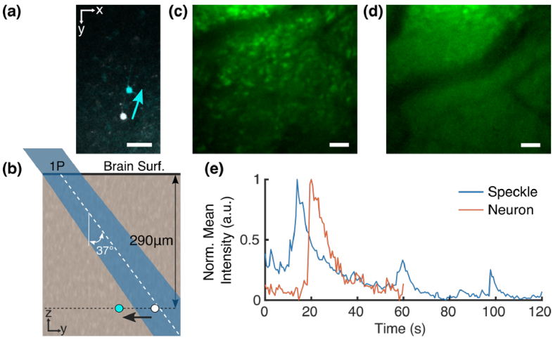
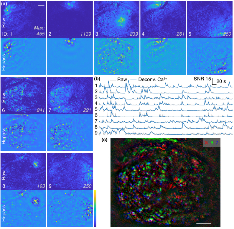
Functional imaging of neuronal activity in awake animals, using a combination of fluorescent reporters of neuronal activity and various types of microscopy modalities, has become an indispensable tool in neuroscience. While various imaging modalities based on one-photon (1P) excitation and parallel (camera-based) acquisition have been successfully used for imaging more transparent samples, when imaging mammalian brain tissue, due to their scattering properties, two-photon (2P) microscopy systems are necessary. In 2P microscopy, the longer excitation wavelengths reduce the amount of scattering while the diffraction-limited 3D localization of excitation largely eliminates out-of-focus fluorescence. However, this comes at the cost of time-consuming serial scanning of the excitation spot and more complex and expensive instrumentation. Thus, functional 1P imaging modalities that can be used beyond the most transparent specimen are highly desirable. Here, we transform light scattering from an obstacle into a tool. We use speckles with their unique patterns and contrast, formed when fluorescence from individual neurons propagates through rodent cortical tissue, to encode neuronal activity. Spatiotemporal demixing of these patterns then enables functional recording of neuronal activity from a group of discriminable sources. For the first time, we provide an experimental, in vivo characterization of speckle generation, speckle imaging and speckle-assisted demixing of neuronal activity signals in the scattering mammalian brain tissue. We found that despite an initial fast speckle decorrelation, substantial correlation was maintained over minute-long timescales that contributed to our ability to demix temporal activity traces in the mouse brain in vivo. Informed by in vivo quantifications of speckle patterns from single and multiple neurons excited using 2P scanning excitation, we recorded and demixed activity from several sources excited using 1P oblique illumination. In our proof-of-principle experiments, we demonstrate in vivo speckle-assisted demixing of functional signals from groups of sources in a depth range of 220-320 µm in mouse cortex, limited by available speckle contrast. Our results serve as a basis for designing an in vivo functional speckle imaging modality and for maximizing the key resource in any such modality, the speckle contrast. We anticipate that our results will provide critical quantitative guidance to the community for designing techniques that overcome light scattering as a fundamental limitation in bioimaging.

Fig. 1.

Schematic illustration of speckle imaging and demixing in the mouse brain. (a) Schematic depiction of three neurons emitting fluorescence, two in the same z-plane and one (green neuron) in a z-plane further away from the brain surface. The green neuron’s plane is denoted as the $Z_i=0$ plane. Two imaging planes are indicated by dashed lines at distances from the green neuron of $Z_i=d_0$ and $Z_i=d_0+d$ , respectively. (b) Schematic illustration of three distinct, partially overlapping and partially developed speckle patterns generated by the neurons in (a), as may be observed when imaging the speckle field at smaller distance $Z_i=d_0$ . (c) Illustration of completely overlapping, fully developed speckle generated by the same three neurons indicated in (a) when imaged at a larger distance, $Z_i=d_0+d$ . Speckle are color-coded according to neuron of origin. (d) Same data as in (c) without color-coding according to neuron of origin. An inverted greyscale is used to ease comparison with (c), i.e., black indicates high brightness. Pronounced brightness is seen in locations where speckle from multiple neurons coincide and interfere constructively. (e) Illustration of three weakly correlated neuronal activity time traces. By spatio-temporal demixing of the corresponding speckle footprints, it is possible to recover the activity time traces, both for partially and fully overlapping speckle fields.

Fig. 2.

Experimental setup for speckle generation by two-photon (2P) excitation. (a) 2P excitation beam path, PMT, detection path, and camera-based detection path, with demagnification stage. Speckle are imaged at different distances $Z_i$ from the objective front focal plane by translating the camera away from the native rear image plane, as indicated. Arrows beside objective illustrate objective translation for focus adjustment of 2P scanning excitation. BS: beamsplitter, DM: dichroic mirror, NBF: 515 nm narrowband filter, WD: objective working distance. All distances are in units of µm. (b) Top panel: Sample raw speckle footprint from a single neuron at depth 415 µm from the brain surface and imaged at $Z_i$  = 590 µm. Inset in bottom left corner: Standard 2P image of the single neuron being scanned, as recorded on the PMT. Bottom panel: Processed version of raw image from the top panel, bandpass-filtered to remove background noise. Scale bar: 50 µm for both top and bottom panels.

Fig. 3.

Speckle contrast versus speckle distance ${\mathit{Z}}_{\mathit{i}}$ . (a) Examples of raw speckle footprints from a single neuron, at four different speckle distances $Z_i$  = 320, 450, 590, and 900 µm. Post-microscope demagnification: 3.75× ( $Z_i$  = 320, 450, 590), 5× ( $Z_i$  = 900 µm). Scale bar: 50 µm. Image size in camera pixels given in upper right corners. (b) Contrast-enhanced and high-pass filtered versions of the images shown in (a), for qualitative visualization of speckle. (c) Fully processed, median- and high-pass-filtered speckle images as used for quantitatively evaluating speckle contrast, with contrast values given in bottom left corners. (d) Speckle contrast as a function of speckle distance $Z_i$ . Two different demagnification optics were used to record the whole range, as indicated in the legend. Data at each $Z_i$ includes at least 6 different neurons from 4 different animals. Gray-shaded area highlights the axial range around the brain surface.

Fig. 4.

Effect of excitation area and detection bandwidth on speckle contrast. (a) Graphical representation of two excitation areas on a single neuron. Area A₁ (20 × 20 µm²) is 16 times larger than area A₂ (5 × 5 µm²) while the total number of pulses in each area was the same. (b) Speckle contrast for two different excitation areas from five different neurons. (c) Speckle contrast for two different fluorescence detection bandwidths, from five different neurons. Excitation area for (c) is ∼3 × 3 µm².

Fig. 5.

Speckle contrast as a function of simultaneously excited neurons. (a-d) Raw speckle footprints from 2P-excited single neurons imaged at $Z_i=590$  µm. Scale bar: 50 µm for all panels. (e) Speckle from neurons 1 and 2 excited simultaneously. (f) Speckle from neurons 3 and 4 excited simultaneously. (g) Three and (h) four neurons excited simultaneously. (i) Lateral locations of neurons 1–4 in the 2p scanning FOV (individual excited areas: 15 × 15 µm). All neurons are at depth 450 µm from the brain surface. Excitation frame rate for individual region-of-interest (ROI) was 60 Hz and 30, 20 and 15 Hz for 2, 3 and 4 ROIs, respectively. (j) Contrast as a function of the number of ROIs (neurons) excited simultaneously. Boxplots include data from four different mice and five distinct regions of imaging. Dashed line: Fit with function $a/\sqrt{N}$ , where N is the number of ROIs. Optimal a = 0.08. R-squared = 0.65.

Fig. 6.

Speckle decorrelation dynamics. (a) Speckle pattern generated by pointing a 2P beam statically at a single neuron; single frame from a 90 s movie recorded at frame rate 501 Hz. Scale bar: 10 camera pixels (camera pixel size: 16 µm). See Visualization 1 for raw data video. (b) Mean image over entire recording. (c) Correlation between mean of initial 200 frames (24 ms) and subsequent frames as a function of time, with linear fits to sliding-window median (red lines; text insets: slope k of linear fits). Yellow trace: unfiltered frames. Blue trace: high-pass-filtered frames (cut-on spatial frequency: 10 pixels per cycle). (d) Second-order autocorrelation function g⁽²⁾ (blue trace) for one pixel from the recording. Inset: same autocorrelation function, zoomed out to longer lag range. Black trace: interpolation between local maxima of g⁽²⁾. Red trace: fit to interpolated data with sum of two exponentials. (e) Heatmap of ratio of g⁽²⁾ at lag 0 and at lag 50 ms for each pixel. (f) Ratio of pixels with pronounced fast decay to less prominent fast decay as a function of neuron depth and distance to nearest in-plane blood vessel. Disk areas indicate ratio, colors are random, for clarity.

Fig. 7.

Oblique one-photon (1P) illumination configuration and fluorescence background rejection. (a) Illustration of oblique collimated excitation beam generated by offsetting an incoming focused beam from the optical axis in the back-focal-plane (BFP) of the objective. (b) 1P beam path characterization using a 3D-suspension of 6-µm fluorescent beads. Background image: YZ-slice from 2P stack, grey scale indicates x coordinate. Overlay: Estimated position of 1P oblique beam. Beam diameter d = 80 µm. Inset: Photo of oblique excitation beam propagating through an agar phantom. (c) Camera image obtained without pinhole for $Z_i=$ 450 µm and objective focal plane at 460 µm depth. Frame is cropped to size of illuminated camera area when no pinhole is in place. Red dashed circle: Location of the 1P beam at brain surface. Blue circle: imaged area with pinhole in place for $Z_i=$ 400 µm. Inset: Image obtained with pinhole in place, showing reduced background.

Fig. 8.

One-photon speckle imaging of a single neuron. (a) Single cropped frame from 2P recording of the target plane (290 µm below brain surface), in grey color scale. The size of the cropped frame roughly coincides with the projection of the oblique region illuminated by the 1P beam on its way into the sample. White spot is the targeted neuron. Overlaid image in cyan color scale: Same as white, but sample shifted by 55 µm to move neuron out of oblique beam as a control as illustrated in (b). Cyan arrow indicates direction of shift of sample for obtaining control measurement. (b) Schematic illustration of 1P illumination path and the single neuron location for speckle excitation (white disk) and control (cyan disk) in an axial section (y-z) view. (c), (d) Standard deviation projections along the time axis of a 2-minute speckle movie recorded on the camera for unshifted (target neuron in excitation region) and shifted (control, target neuron not in excitation region) conditions, (e) Examples of typical neuron activity time series as recorded in standard two-photon imaging (orange trace) and via NMF speckle demixing algorithm (blue trace). Note: Traces represent different recordings, shown at arbitrary offset along horizontal axis. Scale bars: 50 µm

Fig. 9.

Spatio-temporal demixing of 1P-excited speckle from multiple sources. (a) Nine demixed spatial components from mouse cortex, speckle imaging distance Z_i = 300 µm. Raw (top in pair) and high-pass-filtered (bottom in pair) images are shown for each component. High-pass cut-on spatial period: 29.5 µm. White number on left in each pair indicates component number. Number on right indicates maximum brightness value in raw component. Scale bar: 50 µm. Color bar shown right of component 9. (b) Temporal components corresponding to spatial components shown in (a). Gray lines: Raw time traces. Blue line: fits to raw traces constrained by a model of Ca²⁺ dynamics. (c) Enlarged composite image of high-pass-filtered spatial components no. 3 (red), 6 (green), and 7 (blue). Scale bar: 50 µm. See also Supplemental Fig. 1.

References

1. Dana H., Sun Y., Mohar B., et al. , “High-performance calcium sensors for imaging activity in neuronal populations and microcompartments,” Nat. Methods 16(7), 649–657 (2019).10.1038/s41592-019-0435-6 - DOI - PubMed
1. Shemesh O. A., Linghu C., Piatkevich K. D., et al. , “Precision calcium imaging of dense neural populations via a cell-body-targeted calcium indicator,” Neuron 107(3), 470–486.e11 (2020).10.1016/j.neuron.2020.05.029 - DOI - PMC - PubMed
1. Musall S., Kaufman M. T., Juavinett A. L., et al. , “Single-trial neural dynamics are dominated by richly varied movements,” Nat. Neurosci. 22(10), 1677–1686 (2019).10.1038/s41593-019-0502-4 - DOI - PMC - PubMed
1. Kauvar I. V., Machado T. A., Yuen E., et al. , “Cortical observation by synchronous multifocal optical sampling reveals widespread population encoding of actions,” Neuron 107(2), 351–367.e19 (2020).10.1016/j.neuron.2020.04.023 - DOI - PMC - PubMed
1. Conchello J.-A., Lichtman J. W., “Optical sectioning microscopy,” Nat. Methods 2(12), 920–931 (2005).10.1038/nmeth815 - DOI - PubMed
LinkOut - more resources