Exposome-Wide Association Study of Body Mass Index Using a Novel Meta-Analytical Approach for Random Forest Models

Abstract

Background: Overweight and obesity impose a considerable individual and social burden, and the urban environments might encompass factors that contribute to obesity. Nevertheless, there is a scarcity of research that takes into account the simultaneous interaction of multiple environmental factors.

Objectives: Our objective was to perform an exposome-wide association study of body mass index (BMI) in a multicohort setting of 15 studies.

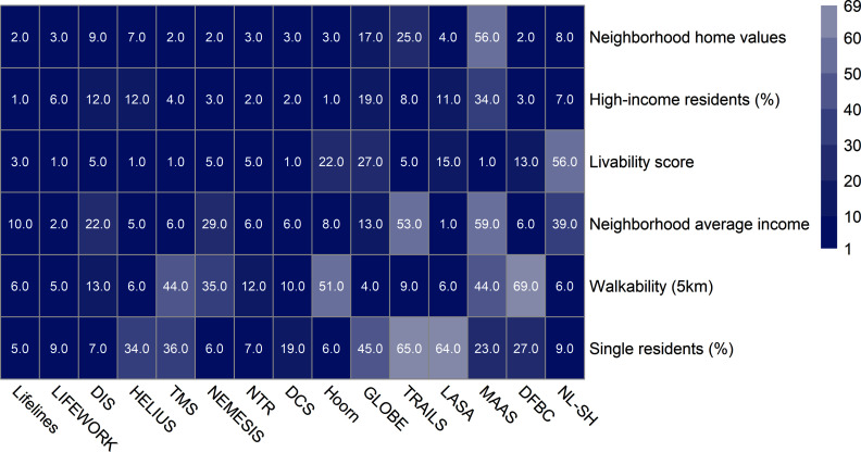
Methods: Studies were affiliated with the Dutch Geoscience and Health Cohort Consortium (GECCO), had different population sizes (688-141,825), and covered the entire Netherlands. Ten studies contained general population samples, others focused on specific populations including people with diabetes or impaired hearing. BMI was calculated from self-reported or measured height and weight. Associations with 69 residential neighborhood environmental factors (air pollution, noise, temperature, neighborhood socioeconomic and demographic factors, food environment, drivability, and walkability) were explored. Random forest (RF) regression addressed potential nonlinear and nonadditive associations. In the absence of formal methods for multimodel inference for RF, a rank aggregation-based meta-analytic strategy was used to summarize the results across the studies.

Results: Six exposures were associated with BMI: five indicating neighborhood economic or social environments (average home values, percentage of high-income residents, average income, livability score, share of single residents) and one indicating the physical activity environment (walkability in $5\text{-km}$ buffer area). Living in high-income neighborhoods and neighborhoods with higher livability scores was associated with lower BMI. Nonlinear associations were observed with neighborhood home values in all studies. Lower neighborhood home values were associated with higher BMI scores but only for values up to $€\mathrm{300,000}$. The directions of associations were less consistent for walkability and share of single residents.

Discussion: Rank aggregation made it possible to flexibly combine the results from various studies, although between-study heterogeneity could not be estimated quantitatively based on RF models. Neighborhood social, economic, and physical environments had the strongest associations with BMI. https://doi.org/10.1289/EHP13393.

Figure 1.

Distributions of ranks of the six most important exposures (see y-axis) associated with body mass index across the 15 cohorts in the Dutch Geoscience and Health Cohort Consortium (GECCO), listed on the x-axis. The lower the value of the ranks, the more important the exposure. The columns are ordered from right to left based on the number of observations in each cohort. Thus, Lifelines had the highest number of participants, and NL-SH had the lowest number. Cohort names and participant numbers are provided in Table 1. Note: DCS, Doetinchem Cohort Study; DFBC, Dutch famine birth cohort; DIS, Donor InSight; GLOBE, Dutch cohort study on socioeconomic health inequalities; HELIUS, Healthy Life in an Urban Setting; LASA, Longitudinal Aging Study Amsterdam; MAAS, Maastricht Aging Study; NEMESIS, Netherlands Mental Health Survey and Incidence Study; NL-SH, Netherlands Longitudinal Study on Hearing; NTR, Netherlands Twin Registry; TMS, The Maastricht Study; TRAILS, Tracking Adolescents’ Individual Lives Survey.

Figure 2.

Shapley plots of neighborhood home values across the studies for each of the cohorts included in the Dutch Geoscience and Health Cohort Consortium (GECCO). Shapley values represent the difference between a prediction and the average prediction of BMI (${\mathrm{kg}/\mathrm{m}}^2$). The size of Shapley values vary; hence, the y-axes are on different scales depending on each cohort. The x-axis represents average administrative neighborhood-level home values, in 1,000s of euros. The solid line represents the smoothed relationship between the observed neighborhood home values and Shapley values for neighborhood home values. Complete cohort names and numbers of participants per cohort are provided in Table 1. Note: BMI, body mass index; DCS, Doetinchem Cohort Study; DFBC, Dutch famine birth cohort; DIS, Donor InSight; GLOBE, Dutch cohort study on socioeconomic health inequalities; HELIUS, Healthy Life in an Urban Setting; LASA, Longitudinal Aging Study Amsterdam; MAAS, Maastricht Aging Study; NEMESIS, Netherlands Mental Health Survey and Incidence Study; NL-SH, National Longitudinal Study on Hearing; NTR, Netherlands Twin Registry; TMS, The Maastricht Study; TRAILS, Tracking Adolescents’ Individual Lives Survey.

Figure 2.

Shapley plots of neighborhood home values across the studies for each of the cohorts included in the Dutch Geoscience and Health Cohort Consortium (GECCO). Shapley values represent the difference between a prediction and the average prediction of BMI (${\mathrm{kg}/\mathrm{m}}^2$). The size of Shapley values vary; hence, the y-axes are on different scales depending on each cohort. The x-axis represents average administrative neighborhood-level home values, in 1,000s of euros. The solid line represents the smoothed relationship between the observed neighborhood home values and Shapley values for neighborhood home values. Complete cohort names and numbers of participants per cohort are provided in Table 1. Note: BMI, body mass index; DCS, Doetinchem Cohort Study; DFBC, Dutch famine birth cohort; DIS, Donor InSight; GLOBE, Dutch cohort study on socioeconomic health inequalities; HELIUS, Healthy Life in an Urban Setting; LASA, Longitudinal Aging Study Amsterdam; MAAS, Maastricht Aging Study; NEMESIS, Netherlands Mental Health Survey and Incidence Study; NL-SH, National Longitudinal Study on Hearing; NTR, Netherlands Twin Registry; TMS, The Maastricht Study; TRAILS, Tracking Adolescents’ Individual Lives Survey.

References

1. WHO (World Health Organization). 2020. Obesity and Overweight. Geneva, Switzerland: WHO. https://www.who.int/news-room/fact-sheets/detail/obesity-and-overweight [accessed 20 January 2021].
1. Wild CP. 2012. The exposome: from concept to utility. Int J Epidemiol 41(1):24–32, PMID: 22296988, 10.1093/ije/dyr236. - DOI - PubMed
1. Chandrabose M, Rachele JN, Gunn L, Kavanagh A, Owen N, Turrell G, et al. . 2019. Built environment and cardio-metabolic health: systematic review and meta-analysis of longitudinal studies. Obes Rev 20(1):41–54, PMID: 30253075, 10.1111/obr.12759. - DOI - PubMed
1. Lam TM, Vaartjes I, Grobbee DE, Karssenberg D, Lakerveld J. 2021. Associations between the built environment and obesity: an umbrella review. Int J Health Geogr 20(1):7, PMID: 33526041, 10.1186/s12942-021-00260-6. - DOI - PMC - PubMed
1. Jia P, Luo M, Li Y, Zheng JS, Xiao Q, Luo J. 2021. Fast-food restaurant, unhealthy eating, and childhood obesity: a systematic review and meta-analysis. Obes Rev 22(suppl 1):e12944, PMID: 31507064, 10.1111/obr.12944. - DOI - PMC - PubMed
Publication types
LinkOut - more resources