SEISMONOISY: A Quasi-Real-Time Seismic Noise Network Monitoring System

Abstract

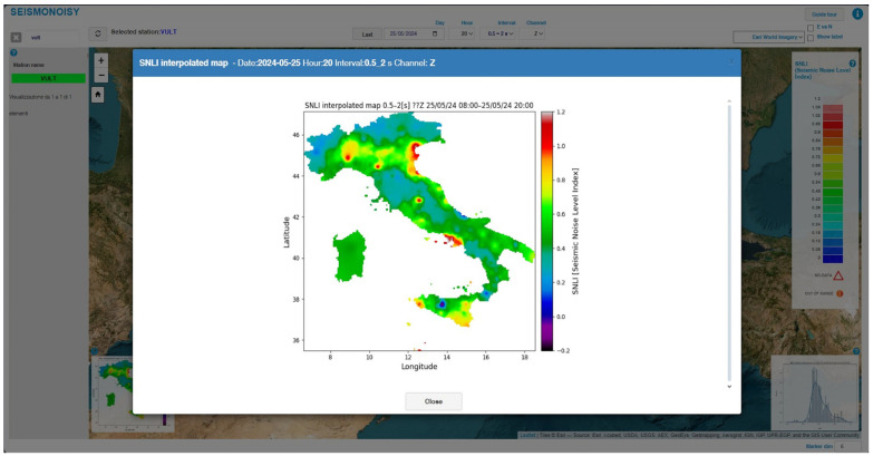
This paper introduces SEISMONOISY, an application designed for monitoring the spatiotemporal characteristic and variability of the seismic noise of an entire seismic network with a quasi-real-time monitoring approach. Actually, we have applied the developed system to monitor 12 seismic networks distributed throughout the Italian territory. These networks include the Rete Sismica Nazionale (RSN) as well as other regional networks with smaller coverage areas. Our noise monitoring system uses the methods of Spectral Power Density (PSD) and Probability Density Function (PDF) applied to 12 h long seismic traces in a 24 h cycle for each station, enabling the extrapolation of noise characteristics at seismic stations after a Seismic Noise Level Index (SNLI), which takes into account the global seismic noise model, is derived. The SNLI value can be used for different applications, including network performance evaluation, the identification of operational problems, site selection for new installations, and for scientific research applications (e.g., volcano monitoring, identification of active seismic sequences, etc.). Additionally, it aids in studying the main noise sources across different frequency bands and changes in the characteristics of background seismic noise over time.

Keywords: background seismic noise level; real time monitoring; seismic noise; seismic noise trend; seismology.

Figure 1

Location map of the different seismic networks and their seismic sensors, taken into account by SEISMONOISY.

Figure 2

Simplified flow diagram of SEISMONOISY application.

Figure 3

Example of result of the PDF function for the station ‘ACER’ belonging to the IV seismic network for the Z component. The blue dash line represents the PSD equal to 50% percentile.

Figure 4

Example of final graph for Z component produced after calculation of the PDF and SNLI. The two black lines, the upper and lower ones, represent the NHNM and NLNM of Peterson’s (1993) curves respectively; the red fill area represents the area between the 50% percentile PDF curve and the NHNM, and the green fill curve represents the area between the 50% percentile PDF curve and the NHNM. The figure also shows the period intervals used to derive the different SNLI values, and the dashed red curve represents noise value characteristic of the seismic sensor installed on the seismic station declared by the manufacturer. Lastly, the blue dashed line represents the PSD value equal to the 50% percentile of the PDF function.

Figure 5

Example of the 50% percentile plot of the PDF function over time in a spectrogram format display for the Z component of station ‘ACER’.

Figure 6

Graphs of the trend of the SNLI value for each period interval for the Z component of the ‘ACER’ station.

Figure 7

Example of the interpolation map of the SNLI value for the interval period 0.5–2 s for the Z component. Since the stations of the seismic networks considered by SEISMONISY are heterogeneous, they are identified with different channel codes. Specifically, the first two letters refer to the properties of the sensor, and the third letter to the channel orientation. For example, HH stands for High Broad Band and High Gain Seismometer sensors, and EH stands for Extremely Short Period and High Gain Seismometer sensors. Since the interpolation map is produced based on both types of sensors, the title of the image indicates ??Z because the interpolation is done with both types of sensors and only the direction is uniquely identified.

Figure 8

Main view of the web users’ interface; this web application allows the users to consult the products generated by the SEISMONOISY application.

Figure 9

Example of the pop-up window opened after clicking on a station, in this case ‘VULT’.

Figure 10

Example of detail of the PDF graph of the station ‘VULT’.

Figure 11

Example of the pop-up window that shows the detailed SNLI interpolation map. The color scale used for this map does not correspond with the range value of the color scale used in the main window (Figure 8), but it is calculated based on the maximum and minimum value of the SNLI value used for interpolation.

Figure 12

The image shows four example PDF function graphs from four different seismic stations (a–d). Each graph highlights potential malfunctions that may be caused by issues of the sensor, the digitizer, or both.

Figure 13

Example of the spectrogram and the graph of the SNLI trend of station (c) reported in Figure 12. From the observation of these two graphs, it is possible to understand when the station began to exhibit anomalous behavior linked to probable malfunctions. For this station, the anomalous behavior started from 30 January 2024.

Figure 14

Examples of different noise contributions related to the different bandwidth of the sensors. In particular, the sensor of the ‘FOSV’ station characterized by a period of 5 s shows an increasingly greater contribution to the noise level at lower frequencies, while the broadband sensors installed at the ‘FDMO’ station show the smallest variation in the noise level in the different period bands.

Figure 15

In the left example of interpolation maps of the seismic level noise expressed in SNLI, on the right, the noise level is measured in the areas of active volcanic context.

Figure 16

Trend of the noise level registered at the ‘OPPE’ station. This station is located in the Po plain in Oppeano town (Verona Province, Italy).

References

1. Havskov J., Alguacil G. Instrumentation in Earthquake Seismology. Modern Approaches in Geophysics. Volume 22. Springer; Dordrecht, The Netherlands: 2004. Seismic networks. - DOI
1. Ringler A.T. Global Seismic Networks: Recording the heartbeat of the Earth. Eos. 2022;103 doi: 10.1029/2022EO225025. - DOI
1. Sahara D.P., Rahsetyo P.P., Nugraha A.D., Syahbana D.K., Widiyantoro S., Zulfakriza Z., Ardianto A., Baskara A.W., Rosalia S., Martanto M., et al. Use of Local Seismic Network in Analysis of Volcano-Tectonic (VT) Events Preceding the 2017 Agung Volcano Eruption (Bali, Indonesia) Front. Earth Sci. 2021;9:619801. doi: 10.3389/feart.2021.619801. - DOI
1. Zheng T., Martin M.P., Sung-Joon C., Hani Z. Evidence for crustal low shear-wave speed in western Saudi Arabia from multi-scale fundamental-mode Rayleigh-wave group-velocity tomography. Earth Planet. Sci. Lett. 2018;495:24–37. doi: 10.1016/j.epsl.2018.05.011. - DOI
1. Quin L., Frank L.V., Christopher W.J., Yehuda B.Z. Spectral Characteristics of Daily to Seasonal Ground Motion at the Piñon Flats Observatory from Coherence of Seismic Data. Bull. Seismol. Soc. Am. 2019;109:1948–1967. doi: 10.1785/0120190070. - DOI
LinkOut - more resources