Modeling the velocity of evolving lineages and predicting dispersal patterns

Abstract

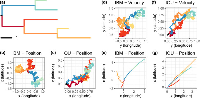
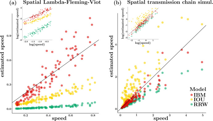
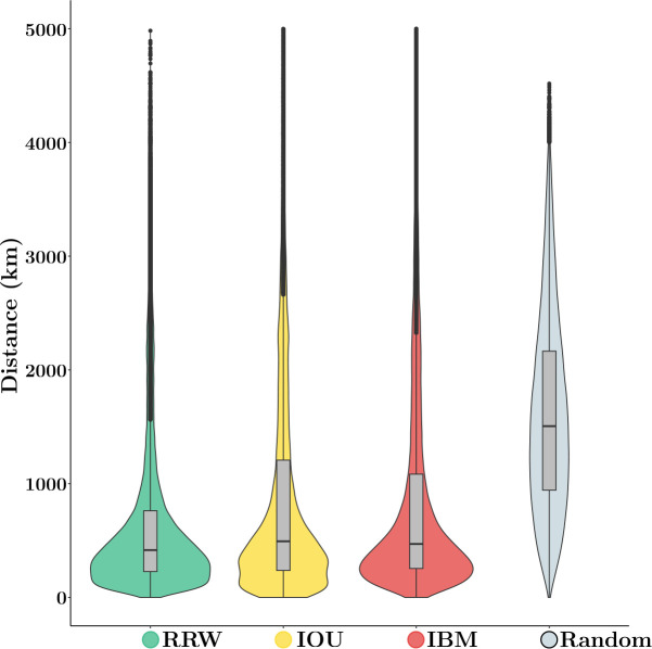
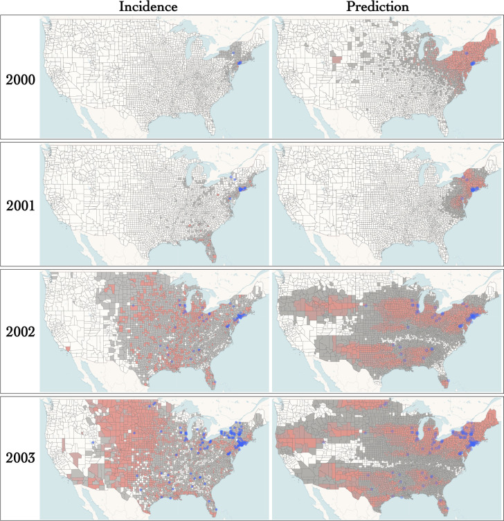
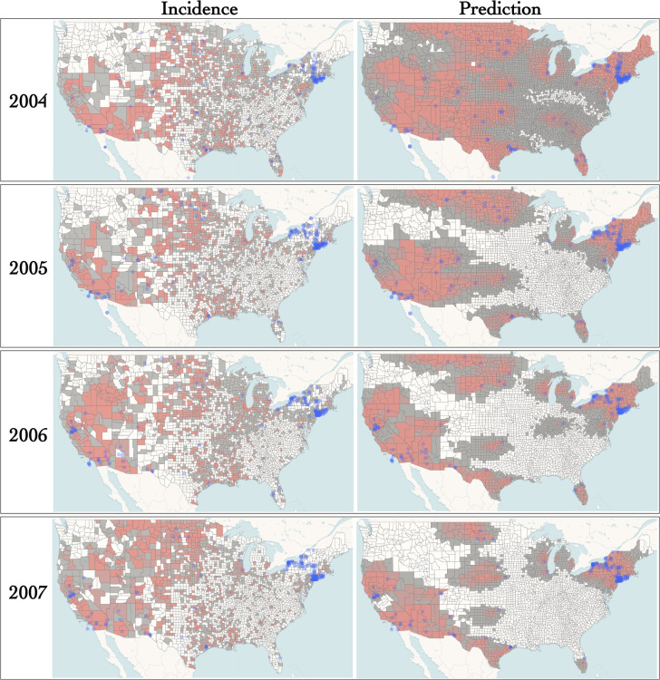
Accurate estimation of the dispersal velocity or speed of evolving organisms is no mean feat. In fact, existing probabilistic models in phylogeography or spatial population genetics generally do not provide an adequate framework to define velocity in a relevant manner. For instance, the very concept of instantaneous speed simply does not exist under one of the most popular approaches that models the evolution of spatial coordinates as Brownian trajectories running along a phylogeny (Lemey et al., 2010). Here, we introduce a new family of models - the so-called "Phylogenetic Integrated Velocity" (PIV) models - that use Gaussian processes to explicitly model the velocity of evolving lineages instead of focusing on the fluctuation of spatial coordinates over time. We describe the properties of these models and show an increased accuracy of velocity estimates compared to previous approaches. Analyses of West Nile virus data in the U.S.A. indicate that PIV models provide sensible predictions of the dispersal of evolving pathogens at a one-year time horizon. These results demonstrate the feasibility and relevance of predictive phylogeography in monitoring epidemics in time and space.

Keywords: BEAST; PhyREX; West Nile virus; integrated velocity models; phylogeography.

Figure 1:. Simulated trajectories of classical random walk and PIV models on a simple tree.

Each process was simulated on the tree (a), with branches of matching colors. Movements along the latitude and longitude axes were simulated independently. (b) Random walk using Brownian motion (BM) with variance ${\sigma }^2=0.1$, and starting point $x\left(0\right)=(0,0)$. (c) Ornstein-Uhlenbeck process (OU) with stationary variance of ${\sigma }^2/\left(2\theta \right)=0.1$, strength $\theta =0.17$, starting at $x\left(0\right)=(0,0)$, and converging to its central value $\mu =(1,1)$. (d) and (e) Velocity $y$ and position $x$ of an Integrated Brownian Motion (IBM) with variance ${\sigma }^2=0.1$, starting point $x\left(0\right)=(0,0)$, and starting velocity $y\left(0\right)=(0,0)$. (f) and (g) Velocity $y$ and position $x$ of an Integrated Ornstein-Uhlenbeck (IOU) with stationary variance ${\sigma }^2/\left(2\theta \right)=0.1$, strength $\theta =0.17$, central trend of $\mu =(1,1)$, starting point $x\left(0\right)=(0,0)$, and starting velocity $y\left(0\right)=(0,0)$.

Figure 2:. Accuracy of speed estimation under the RRW and PIV models.

True (x-axis) vs. estimated (y-axis) speed. Estimates were obtained under the IBM, IOU and RRW models. (a) 100 data sets were simulated using the spatial Lambda-Fleming-Viot process on a 10 by 10 square. (b) 100 data sets were simulated under a random walk model inspired by the Ebola epidemic in West Africa (see main text). The insets give the log-log scatterplots of the estimated vs. true speeds. The $y=x$ line is shown in black on each plot.

Figure 3:. Distribution of the distance between true and estimated tip coordinates under the PIV, the RRW models and uniform at random predictions, WNV data.

Cross validation was used to predict the locations of held-one-out tip lineages under the RRW and PIV models. ‘Random’ gives the distance between two locations selected uniformly at random within the U.S.A. The y axis gives the great circle distance between coordinates (in km).

Figure 4:. Incidence and predicted occurrence of WNV in the early phase of the epidemic (model for prediction: IBM).

Purple dots correspond to sampled locations. Incidence data (left) for each year and each county was obtained from the CDC. For year , predicted occurrence of the WNV (right) was inferred using data collected earlier than the end of December of year $Y-1$. The maps were generated with EvoLaps2 (Chevenet et al., 2024)

Figure 5:. Incidence and predicted occurrence of WNV in an endemic regime (model for prediction: IBM).

See caption of Fig. 4.

References

-
- Baele G., Dellicour S., Suchard M., Lemey P., and Vrancken B. 2018. Recent advances in computational phylodynamics. Current Opinion in Virology, 31: 24–32. - PubMed
- Barndorff-Nielsen O. and Shephard N. 2003. Integrated OU processes and non-Gaussian OU-based stochastic volatility models. Scandinavian Journal of Statistics, 30: 277–295.
- Barton N., Etheridge A., and Véber A. 2010. A new model for evolution in a spatial continuum. Electronic Journal of Probability, 15: 162–216.
- Barton N., Etheridge A., and Véber A. 2013. Modelling evolution in a spatial continuum. Journal of Statistical Mechanics: Theory and Experiment, 2013: P01002.
Publication types
Grants and funding
LinkOut - more resources
Full Text Sources