Machine learning of dissection photographs and surface scanning for quantitative 3D neuropathology

Abstract

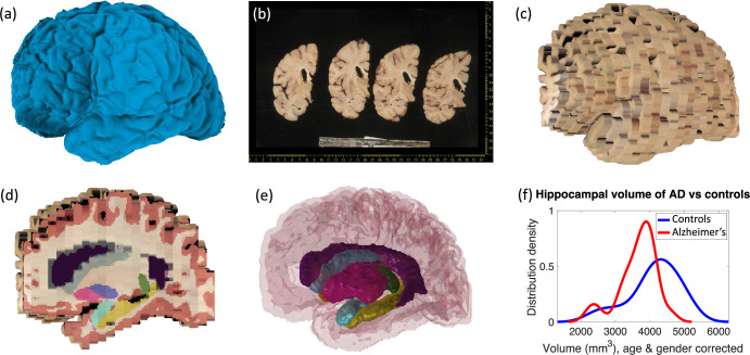
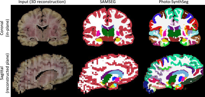
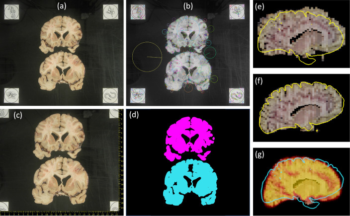
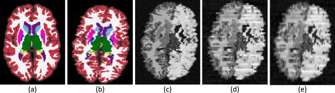
We present open-source tools for three-dimensional (3D) analysis of photographs of dissected slices of human brains, which are routinely acquired in brain banks but seldom used for quantitative analysis. Our tools can: (1) 3D reconstruct a volume from the photographs and, optionally, a surface scan; and (2) produce a high-resolution 3D segmentation into 11 brain regions per hemisphere (22 in total), independently of the slice thickness. Our tools can be used as a substitute for ex vivo magnetic resonance imaging (MRI), which requires access to an MRI scanner, ex vivo scanning expertise, and considerable financial resources. We tested our tools on synthetic and real data from two NIH Alzheimer's Disease Research Centers. The results show that our methodology yields accurate 3D reconstructions, segmentations, and volumetric measurements that are highly correlated to those from MRI. Our method also detects expected differences between post mortem confirmed Alzheimer's disease cases and controls. The tools are available in our widespread neuroimaging suite 'FreeSurfer' (https://surfer.nmr.mgh.harvard.edu/fswiki/PhotoTools).

Keywords: dissection photography; human; machine learning; neuroscience; surface scanning; volumetry.

Figure 1.. Examples of inputs and outputs from the MADRC dataset.

(a) Three-dimensional (3D) surface scan of left human hemisphere, acquired prior to dissection. (b) Routine dissection photography of coronal slabs, after pixel calibration, with digital rulers overlaid. (c) 3D reconstruction of the photographs into an imaging volume. (d) Sagittal cross-section of the volume in (c) with the machine learning segmentation overlaid. The color code follows the FreeSurfer convention. Also, note that the input has low, anisotropic resolution due to the large thickness of the slices (i.e., rectangular pixels in sagittal view), whereas the 3D segmentation has high, isotropic resolution (squared pixels in any view). (e) 3D rendering of the 3D segmentation into the different brain regions, including hippocampus (yellow), amygdala (light blue), thalamus (green), putamen (pink), caudate (darker blue), lateral ventricle (purple), white matter (white, transparent), and cortex (red, transparent). (f) Distribution of hippocampal volumes in post mortem confirmed Alzheimer’s disease vs controls in the MADRC dataset, corrected for age and gender.

Figure 2.. Qualitative comparison of SAMSEG vs Photo-SynthSeg: coronal (top) and sagittal (bottom) views of the reconstruction and automated segmentation of a sample whole brain from the UW-ADRC dataset.

Note that Photo-SynthSeg supports subdivision of the cortex with tools of the SynthSeg pipeline.

Figure 3.. Dice scores of automated vs manual segmentations on select slices.

Box plots are shown for SAMSEG, Photo-SynthSeg, and two ablations: use of probabilistic atlas and targeted simulation with 4 mm slice spacing. Dice is computed in two-dimensional (2D), using manual segmentations on select slices. We also note that the absence of extracerebral tissue in the images contributes to high Dice for the cortex.

Figure 4.. Reconstruction error (in mm) in synthetically sliced HCP data.

The figure shows box plots for the mean reconstruction error as a function of spacing and thickness jitter. A jitter of $j$ means that the n^th slice is randomly extracted from the interval $[n-j,n+j]$ (rather than exactly $n$). The center of each box represents the median; the edges of the box represent the first and third quartiles; and the whiskers extend to the most extreme data points not considered outliers (not shown, in order not to clutter the plot).

Figure 5.. Steps of proposed processing pipeline.

(a) Dissection photograph with brain slices on black board with fiducials. (b) Scale-invariant feature transform (SIFT) features for fiducial detection. (c) Photograph from (a) corrected for pixel size and perspective, with digital ruler overlaid. (d) Segmentation against the background, grouping pieces of tissue from the same slice. (e) Sagittal slice of the initialization of a three-dimensional (3D) reconstruction. (f) Corresponding slice of the final 3D reconstruction, obtained with a surface as reference (overlaid in yellow). (g) Corresponding slice of the 3D reconstruction provided by a probabilistic atlas (overlaid as a heat map); the real surface is overlaid in light blue for comparison.

Figure 6.. Intermediate steps in the generative process.

(a) Randomly sampled input label map from the training set. (b) Spatially augmented input label map; imperfect 3D reconstruction is simulated with a deformation jitter across the coronal plane. (c) Synthetic image obtained by sampling from a Gaussian mixture model conditioned on the segmentation, with randomized means and variances. (d) Slice spacing is simulated by downsampling to low resolution. This imaging volume is further augmented with a bias field and intensity transforms (brightness, contrast, gamma). (e) The final training image is obtained by resampling (d) to high resolution. The neural network is trained with pairs of images like (e) (input) and (b) (target).

Appendix 1—figure 1.. Simulation and reconstruction of synthetic data.

Top row: skull stripped T1 scan and (randomly translated and rotated) binary mask of the cerebrum, in yellow. Second row: original T2 scan. Third row: randomly sliced and linearly deformed T2 images. Bottom row: output of the 3D reconstruction algorithm, that is, reconstructed T2 slices and registered reference mask overlaid in yellow.

Appendix 1—figure 2.. Reconstruction with surface scan vs probabilistic atlas.

(a) Initialization, with contour of 3D surface scan superimposed. (b) Reconstruction with 3D surface scan. (c) Reconstruction with probabilistic atlas (overlaid as heat map with transparency); the contour of the surface scan is overlaid in light blue, for comparison. Even though the shape of the reconstruction in (c) is plausible, it is clearly inaccurate in light of the surface scan.

Appendix 1—figure 3.. Example of mid-coronal slice selected for manual segmentation and computation of Dice scores.

Compared with the FreeSurFer protocol, we merge the ventral diencephalon (which has almost no visible contrast in the photographs) with the cerebral white matter in our manual delineations. We also merged this structures in the automated segmentations from SAMSEG and Photo-SynthSeg in this figure, for a more consistent comparison.

References

-
- Abadi M, Barham P, Chen J, Chen Z, Davis A. Tensorflow: A system for large-scale machine learning. Symposium on Operating Systems Design and Implementation; 2016. pp. 265–283.
- Billot B, Greve D, Van Leemput K, Fischl B, Iglesias JE, Dalca A. A Learning Strategy for Contrast-agnostic MRI Segmentation. Medical Imaging with Deep Learning; 2020. pp. 75–93.
MeSH terms
Grants and funding
- U01MH117023/NH/NIH HHS/United States
- R01EB031114/NH/NIH HHS/United States
- R01NS083534/NH/NIH HHS/United States
- R01 MH121885/NH/NIH HHS/United States
- R01 MH123195/NH/NIH HHS/United States
- R01 EB023281/EB/NIBIB NIH HHS/United States
- R01 AG008122/AG/NIA NIH HHS/United States
- R01EB019956/NH/NIH HHS/United States
- Grant Ref 2021UPC-MS-67573/Politècnica de Catalunya
- U01 MH093765/MH/NIMH NIH HHS/United States
- R01 NS070963/NS/NINDS NIH HHS/United States
- U01 NS086625/NS/NINDS NIH HHS/United States
- R21 EB018907/EB/NIBIB NIH HHS/United States
- ARUK-IRG2019A-003/Alzheimer's Research UK
- R21NS072652/NH/NIH HHS/United States
- R01 AG064027/AG/NIA NIH HHS/United States
- 1S10RR023043/NH/NIH HHS/United States
- R01 AG016495/AG/NIA NIH HHS/United States
- P30 AG062421/AG/NIA NIH HHS/United States
- 1R01EB023281/NH/NIH HHS/United States
- R01AG016495/NH/NIH HHS/United States
- R01 NS112161/NS/NINDS NIH HHS/United States
- S10 RR019307/RR/NCRR NIH HHS/United States
- R01NS112161/NH/NIH HHS/United States
- R01 AG070988/AG/NIA NIH HHS/United States
- P30AG066509 (UW ADRC)/NH/NIH HHS/United States
- RF1 MH123195/MH/NIMH NIH HHS/United States
- 1S10RR019307/NH/NIH HHS/United States
- R01EB006758/NH/NIH HHS/United States
- R01AG070988/AG/NIA NIH HHS/United States
- RF1 MH121885/MH/NIMH NIH HHS/United States
- 5U01NS086625/NH/NIH HHS/United States
- R01NS105820/NH/NIH HHS/United States
- R01 NS105820/NS/NINDS NIH HHS/United States
- 1R56AG064027/NH/NIH HHS/United States
- 1R01AG070988/NH/NIH HHS/United States
- K08AG065426/NH/NIH HHS/United States
- U19 AG060909/AG/NIA NIH HHS/United States
- 1RF1MH123195/NH/NIH HHS/United States
- 5R01AG008122/NH/NIH HHS/United States
- P30 AG066509/AG/NIA NIH HHS/United States
- ERC Starting Grant 677697/European Union
- P30AG062421/AG/NIA NIH HHS/United States
- U19AG066567/NH/NIH HHS/United States
- R01 EB019956/EB/NIBIB NIH HHS/United States
- R56 AG064027/AG/NIA NIH HHS/United States
- K08 AG065426/AG/NIA NIH HHS/United States
- P41EB030006/NH/NIH HHS/United States
- 5U01MH093765/NH/NIH HHS/United States
- P41 EB030006/EB/NIBIB NIH HHS/United States
- R01 EB031114/EB/NIBIB NIH HHS/United States
- 1R01AG064027/NH/NIH HHS/United States
- 5U24NS10059103/NH/NIH HHS/United States
- R01NS070963/NH/NIH HHS/United States
- U19AG060909/NH/NIH HHS/United States
- U01 MH117023/MH/NIMH NIH HHS/United States
- R21 NS072652/NS/NINDS NIH HHS/United States
- UM1MH130981/NH/NIH HHS/United States
- S10 RR023043/RR/NCRR NIH HHS/United States
- 1S10RR023401/NH/NIH HHS/United States
- U19 AG066567/AG/NIA NIH HHS/United States
- RF1MH123195/NH/NIH HHS/United States
- R21EB018907/NH/NIH HHS/United States
- R01 EB006758/EB/NIBIB NIH HHS/United States
- R01 NS083534/NS/NINDS NIH HHS/United States
- S10 RR023401/RR/NCRR NIH HHS/United States
- R01NS0525851/NH/NIH HHS/United States
- UM1 MH130981/MH/NIMH NIH HHS/United States
LinkOut - more resources
Full Text Sources
Medical
Miscellaneous