THE ECONOMIC IMPACTS OF COVID-19: EVIDENCE FROM A NEW PUBLIC DATABASE BUILT USING PRIVATE SECTOR DATA

Abstract

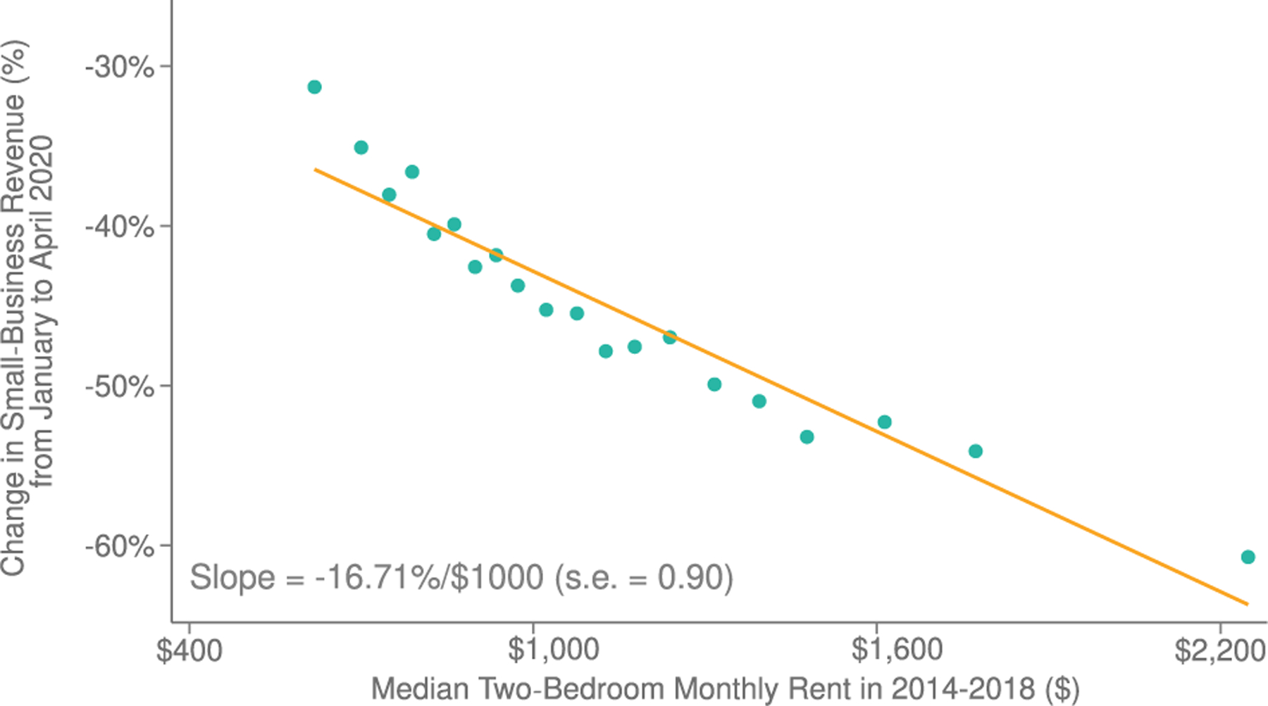
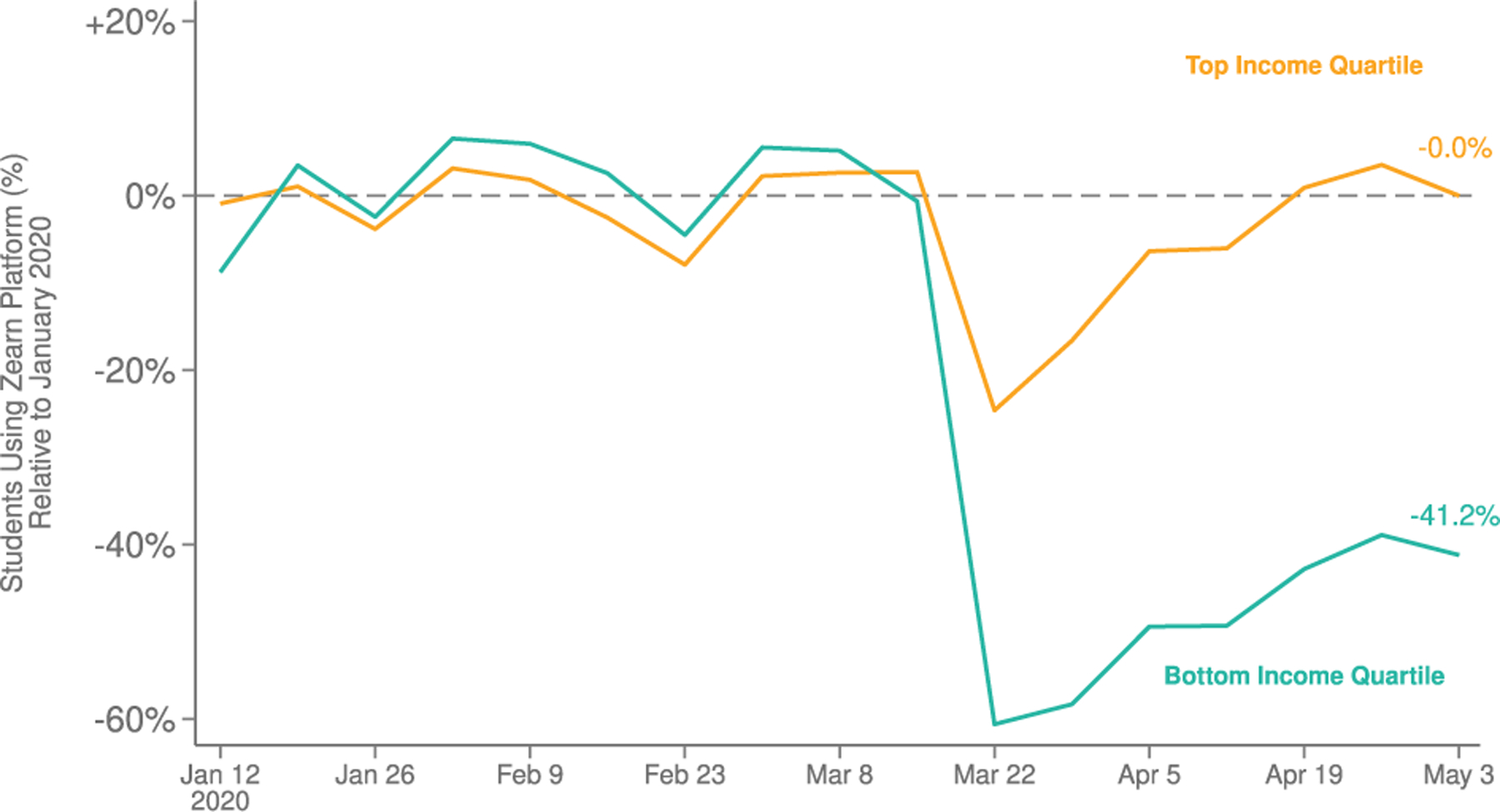
We build a publicly available database that tracks economic activity in the United States at a granular level in real time using anonymized data from private companies. We report weekly statistics on consumer spending, business revenues, job postings, and employment rates disaggregated by county, sector, and income group. Using the publicly available data, we show how the COVID-19 pandemic affected the economy by analyzing heterogeneity in its effects across subgroups. High-income individuals reduced spending sharply in March 2020, particularly in sectors that require in-person interaction. This reduction in spending greatly reduced the revenues of small businesses in affluent, dense areas. Those businesses laid off many of their employees, leading to widespread job losses, especially among low-wage workers in such areas. High-wage workers experienced a V-shaped recession that lasted a few weeks, whereas low-wage workers experienced much larger, more persistent job losses. Even though consumer spending and job postings had recovered fully by December 2021, employment rates in low-wage jobs remained depressed in areas that were initially hard hit, indicating that the temporary fall in labor demand led to a persistent reduction in labor supply. Building on this diagnostic analysis, we evaluate the effects of fiscal stimulus policies designed to stem the downward spiral in economic activity. Cash stimulus payments led to sharp increases in spending early in the pandemic, but much smaller responses later in the pandemic, especially for high-income households. Real-time estimates of marginal propensities to consume provided better forecasts of the impacts of subsequent rounds of stimulus payments than historical estimates. Overall, our findings suggest that fiscal policies can stem secondary declines in consumer spending and job losses, but cannot restore full employment when the initial shock to consumer spending arises from health concerns. More broadly, our analysis demonstrates how public statistics constructed from private sector data can support many research and real-time policy analyses, providing a new tool for empirical macroeconomics.

Keywords: E01; E32.

FIGURE I

Changes in Consumer Spending during the COVID Pandemic This figure disaggregates spending changes by income and sector using debit and credit card data from Affinity Solutions and national accounts (NIPA) data. Panel A plots daily spending levels for consumers in the highest and lowest quartiles of household income by combining total card spending in January 2020 (from NIPA Table 2.3.5) with our Affinity Solutions spending series. See the notes to Online Appendix Table V for details on this method. Panel B disaggregates the sectoral shares of seasonally adjusted spending changes (left bar) and pre-COVID spending levels (right bar). See Online Appendix B.3 for the definitions of the sectors plotted in Panel B. Panel C decomposes the change in personal consumption expenditures (PCE) in the Great Recession and the COVID-19 recession using NIPA Table 2.3.6. PCE is defined here as the sum of durable goods, nondurable goods, and services in seasonally adjusted, chained (2012) dollars. The peak to trough declines are calculated from December 2007 to June 2009 for the Great Recession and from January to April 2020 for the COVID-19 recession. Data sources: Affinity Solutions, NIPA.

FIGURE II

Association between COVID-19 Incidence and Changes in Consumer Spending This figure presents a county-level binned scatter plot. To construct it, we divide the data into 20 equal-sized bins, ranking by the x-axis variable and weighting by the county’s population, and plot the (population-weighted) means of the y-axis and x-axis variables in each bin. The y-axis presents the change in seasonally adjusted consumer spending from the base period (January 6–February 2, 2020) to the three-week period of March 25 to April 14, 2020 (see Section II.B and Online Appendix B for details on the construction of our consumer spending series). The x-axis variable is the log of the county’s cumulative COVID case rate per capita as of April 14, 2020; axis labels show the levels on a log scale. We plot values separately for counties in the top and bottom quartiles of median household income (measured using population-weighted 2014–2018 ACS data). Data sources: Affinity Solutions, New York Times.

FIGURE III

Changes in Small-Business Revenues versus Median Two-Bedroom Rent, by ZIP Code This figure presents a binned scatter plot showing the relationship between changes in seasonally adjusted small-business revenue in Womply data versus rent at the ZIP code level. The binned scatter plot is constructed as described in Figure II. We measure changes in small-business revenue as the average value of our index at the ZIP code level between March 23 and April 12, 2020 (see Section II.B and Online Appendix C for details on the construction of our small-business revenue series). The x-axis variable is the ZIP code median rent for a two-bedroom apartment in the 2014–2018 ACS. Data sources: Womply, ACS.

FIGURE IV

Changes in Job Postings and Employment Rates versus Rent This figure shows binned scatter plots of the relationship between median rents and changes in job postings (Panels A and B) or changes in employment rates (Panel C). The binned scatter plots are constructed as described in Figure II. Solid lines are best-fit lines estimated using OLS. Each panel also displays the slope coefficient and standard error of the corresponding linear OLS regression. In each panel, the x-axis variable is the median rent in a county for a two-bedroom apartment in the 2014–2018 ACS. In Panel A, the y-axis variable is the average value of our job postings series for jobs requiring minimal or some education between March 25 and April 14, 2020 (see Section II.B and Online Appendix D for more detail on our job postings series). Panel B replicates Panel A with job postings for workers with moderate, considerable, or extensive education. In both Panels A and B, we winsorize our job postings series at the 99th percentile of the (population-weighted) county-level distribution within each level of required education. In Panel C, the y-axis variable is the average value of our bottom wage quartile employment series during July 2020 (see Section II.B and Online Appendix E for more detail on the construction of our employment series). Data sources: Paychex, Intuit, Lightcast, ACS.

FIGURE V

Changes in Employment by Wage Quartile Panel A plots our combined Paychex-Intuit employment series from January 2020 through December 2021 for each wage quartile. We define moving wage quartile thresholds in each month based on 100%, 150%, and 250% of the federal poverty line for a family of four, adjusted for inflation, then converted into a full-time-equivalent hourly wage by dividing by 2,000 hours (50 weeks of work at 40 hours per week). In January 2020, the thresholds were $13.10, $19.65, and $32.75, and the four bins in ascending order by wage contained 23.4%, 27.4%, 25.7%, and 23.5% of CPS respondents. See Section II.B and Online Appendix E for details on the construction of this series. In Panel B, we reweight the county-by-industry (two-digit NAICS) distribution of bottom wage quartile employment to match the distribution for top wage quartile employment in January 2020. For each series in Panel B, we restrict the sample to county-by-industry cells with nonzero employment in all four wage quartiles in January 2020; this sample restriction excludes 2.5% of worker-days from the sample. Data sources: Paychex, Intuit.

FIGURE VI

Evolution of the Association between Low-Education Job Postings and Low-Wage Employment with Rent This figure presents a summary of the results of a set of regressions documenting the relationship between job postings and employment with rent over time. Panel A replicates Figure IV, Panel A, but using the average value of the low-education job postings series in December 2021 instead of April 2020. Panel B replicates Figure IV, Panel C, but using the average value of the Paychex-Intuit employment series in December 2021 instead of July 2020. The binned scatter plots are constructed as described in Figure II. Panel C plots the slope of the best-fit line from a population-weighted regression of low-education job postings on median county rent (as in Panel A) for each month from April 2020 through December 2021. The slopes estimated in Figures IV, Panel A and VI, Panel A are the first and last estimates in this series, respectively. Panel D replicates Panel C for the slope of the bottom wage quartile employment versus median rent (as in Panel B). In Panels C and D, the dashed lines above and below the solid series represent the upper and lower boundaries of the 95% confidence interval for the slope estimated in each month. Panels B and D omit counties from CA, MA, and NY, since these three states raised the minimum wage at some point after July 2020 above our upper threshold for the bottom wage quartile of employment. Data sources: Lightcast, Paychex, Intuit, ACS.

FIGURE VII

Effects of Stimulus Payments on Spending: Event Studies This figure shows event studies of the effect of stimulus payments on consumer spending. We measure consumer spending using data from Affinity Solutions. To construct each consumer spending time series, we express consumer spending on each day as a percentage change relative to mean daily consumer spending over January 2019, residualize these daily percentage changes with respect to day-of-week fixed effects (estimated out-of-sample using data in 2019), calculate the first difference with respect to values from the corresponding period starting in 2019, and adjust the estimates for a linear pretrend in first differences. Panel A depicts this spending time series for 25 days before and after April 15, 2020 (the modal date for deposits of the CARES Act economic impact payments) for cardholders with residential addresses in the bottom income quartile of ZIP codes. We exclude April 14, 2020, from the preperiod because some households received stimulus payments on this date. Panel B repeats this figure for the top income quartile of ZIP codes. Panel C repeats Panels A and B for the days around January 4, 2021 (the modal date for deposits of the COVID-Related Tax Relief Act economic impact payments), plotting outcomes for both the bottom and top income quartiles. The preperiod in Panel C runs from December 4 to 14, 2020, with the holiday period (December 15, 2020 to January 3, 2021) removed due to high daily volatility in spending levels (see Section IV.A and Online Appendix Figure XXIII for more details). The postperiod runs from January 4 to 19, 2021, reflecting the data available when this analysis was originally published on January 26, 2021. Due to the omission of the holiday period, we do not remove a linear pretrend as in Panels A and B. Panel D repeats Panel C for the days around March 17, 2021 (the modal date for deposits of the American Rescue Plan Act economic impact payments). We exclude March 13 to 16, 2021 from the preperiod as payments were made starting March 13. In Panels A, B, and D, we interpolate the value for Easter Sunday using the average of adjacent daily values. Data sources: Affinity Solutions, ACS.

FIGURE VIII

Impacts of Stimulus Payments on Spending, by Income Quartile This figure plots estimates of the marginal propensity to spend out of stimulus payments in the first month after receipt for each of the three rounds of stimulus payments, separately by income quartile (based on median ZIP code income). The estimates are scaled per $1,200 of stimulus payment and correspond to the “Combined Dollar” estimates reported in Online Appendix Table VI, column (5). See Section IV.A and Online Appendix K.3 for details on how these estimates were calculated. We also report p-values testing the null hypothesis of equal effect sizes between each pair of stimulus rounds, for the highest- and lowest-quartile of ZIP-level incomes. These p-values are based on permutation tests reported in Online Appendix Figures XXIV and XXV. Data source: Affinity Solutions.

FIGURE IX

Changes in Employment and Consumer Spending for Low-Income Households versus Workplace Rent This figure examines the relationship between low-wage employment and consumer spending for individuals living in a home ZIP code z with the average rent in the ZIP codes of the workplaces for low-wage workers who live in home ZIP code z. Panel A presents a binned scatterplot showing the relationship between low-wage employment for workers living in a home ZIP code and the average median rent in the workplace ZIP codes for low-wage workers from that home ZIP code. We measure low-wage employment in each home ZIP code using the Earnin employment series in April 2020. We then match each home ZIP code to the distribution of workplace ZIP codes using the Census LODES data for low-wage workers. We calculate the x-axis variable as the average median rent for a two-bedroom apartment (measured in the 2014–2018 ACS), averaged across workplace ZIP codes using the distribution from the LODES data for each home ZIP code. See Section IV.C for a detailed discussion. Panel B replicates Panel A for a different outcome: average consumer spending between March 25 and April 14, 2020, restricting to ZIP codes in the bottom quartile of median income, as measured in the 2014–2018 ACS. Panel C replicates Panel B with consumer spending instead measured during October 2020. The binned scatter plots are constructed as described in Figure II. Panel D plots the average level of consumer spending for the top quartile of households appearing in Panels B and C ranked on average median workplace rent (i.e., the five right-most dots) in each month from February 2020 through December 2021. Data sources: Earnin, Affinity Solutions, Census LODES, ACS.

FIGURE X

Effects of COVID-19 on Educational Progress by Income Group This figure plots a time series of student engagement on the Zearn Math online platform, splitting schools into quartiles based on the share of students in the school eligible for Free or Reduced Price Lunch (FRPL). We measure student engagement as the average number of students using the Zearn Math application in each week, relative to the mean value of students using the platform in the same classroom during the reference period of January 6 to February 7, 2020. We restrict the sample to classrooms with at least 10 students using Zearn on average and at least 5 students doing so in each week during the reference period. We measure the share of students eligible for FRPL in each school using demographic data from the Common Core data set from MDR Education, a private education data firm. Data sources: Zearn, Common Core.

References

1. Abraham Katharine G., Jarmin Ron S., Moyer Brian, and Shapiro Matthew D., eds., Big Data for 21st Century Economic Statistics, (Chicago: University of Chicago Press, 2019).
1. Aldy Joseph E., “The Labor Market Impacts of the 2010 Deepwater Horizon Oil Spill and Offshore Oil Drilling Moratorium,” NBER Working Paper no. 20409, 2014. 10.3386/w20409 - DOI
1. Alexander Diane, and Karger Ezra, “Do Stay-at-Home Orders Cause People to Stay at Home? Effects of Stay-at-Home Orders on Consumer Behavior,” Review of Economics and Statistics, 105 (2023), 1017–1027. 10.1162/rest_a_01108 - DOI
1. Allcott Hunt, Boxell Levi, Conway Jacob, Gentzkow Matthew, Thaler Michael, and Yang David, “Polarization and Public Health: Partisan Differences in Social Distancing during the Coronavirus Pandemic,” Journal of Public Economics, 191 (2020), 104254. 10.1016/j.jpubeco.2020.104254 - DOI - PMC - PubMed
1. An Xudong, Gabriel Stuart A., and Tzur-Ilan Nitzan, “More Than Shelter: The Effect of Rental Eviction Moratoria on Household Well-Being,” AEA Papers and Proceedings, 112 (2022), 308–312. 10.1257/pandp.20221108 - DOI
LinkOut - more resources