Visual neurons recognize complex image transformations

Abstract

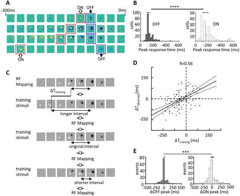
Natural visual scenes are dominated by sequences of transforming images. Spatial visual information is thought to be processed by detection of elemental stimulus features which are recomposed into scenes. How image information is integrated over time is unclear. We explored visual information encoding in the optic tectum. Unbiased stimulus presentation shows that the majority of tectal neurons recognize image sequences. This is achieved by temporally dynamic response properties, which encode complex image transitions over several hundred milliseconds. Calcium imaging reveals that neurons that encode spatiotemporal image sequences fire in spike sequences that predict a logical diagram of spatiotemporal information processing. Furthermore, the temporal scale of visual information is tuned by experience. This study indicates how neurons recognize dynamic visual scenes that transform over time.

Fig. 1.. Tectal cell visual response properties change over time

A. Recording setup. Animals were placed on a stage in the center of a recording chamber equipped with a rear-projector screen on the side of the chamber. Black and white squares represent stimuli used to identify tectal cell response properties. Neuronal activity was recorded with juxtacellular glass electrodes in response to an unbiased sparse noise visual stimulation protocol, consisting of 4000-16000 randomly generated images of combinations of two white or black squares on a gray background, presented for 400-600ms without a gap. B. Spatiotemporal response properties change over time, displayed as a Spike Triggered Average (STA). (top) Polar spatiotemporal responses, showing increasing complexity of optimal stimuli from one, two, three or more poles. (bottom) Categories of temporal response dynamics. Shift: parallel shift without changing the vector of ON to OFF poles. Rotate: two examples in which the vector connecting ON and OFF poles spins. Complex: other complex changes, such as changes in distributed ON and OFF responses over time. C. Percentages of spatial patterns (right) and temporal patterns (left).

Fig. 2.. Tectal neurons detect direction selective rotating stimuli

A. Unbiased stimulus presentation identifies rotation as an optimal stimulus. Top: RF maps determined by reverse correlation analysis. Bottom: The axis connecting ON-OFF RF centers (red and blue, respectively) rotated over time. bin: 25ms. Values below RF maps are the ending timepoints of the 25 ms bins. Color scale: spike numbers normalized to the absolute maximum value. B. Stimuli used to test direction selectivity of the rotation response. A counterclockwise (CCW, top) or clockwise (CW, bottom) rotating circular gradient was presented in the RF. C. Number of spikes evoked by the rotating image at different speeds from two representative neurons shows directional selectivity for rotation. (left) An example of preference for CW rotation (magenta) compared to CCW (blue). (right) A neuron in which the preferred rotation direction showed speed-dependent switching between CCW (blue) and CW (magenta) rotation. Responses to CW and CCW rotation were significantly different at several rotation speeds. * p< 0.05, *** p< 0.001 bootstrap test, 10⁵ repeats, n=6 sessions. D. Percentages of neurons showing significant rotation direction selectivity (n=15 units). Neurons with P[#Spikes(CW)=#Spikes(CCW)]<0.05 and ∣DSI∣≥0.1 at any rotation speed are counted as rotation direction selective. E. Cumulative distribution of rotational direction selectivity index at the optimal speed. (n=38 units). F-G. Rotation direction selectivity is not achieved by the summation of responses to a series of linear direction selective stimuli. F. Sets of stimuli to evaluate summation of linear direction selective responses. Drifting gratings were presented in semicircles of 12 orientations in the cell’s RF in CCW (blue) and CW (magenta) directions. G. Total number of spikes evoked by the sets of linear CW or CCW motion stimuli. DSI = 0.020 (600deg/s), 0.033 (900deg/s), 0.025(1200deg/s), −0.018 (1500deg/s). Compare with responses of the same cell to rotational stimuli (C, left).

Fig. 3.. Tectal neurons recognize sequence-specific image transitions.

A. RF maps of visually-evoked response dynamics over time determined by reverse correlation analysis. ON and OFF responses are shown in yellow and blue, respectively. The image sequence that evoked this response is termed the “original” sequence. B. Analysis of stimulus sequence specificity of visual response properties. (i) Sequence of frame numbers for the original and reverse stimulus sequences and a representative sequence of shuffled stimuli (blue, magenta and black respectively). (ii) Temporal profiles of responses to original, reverse and shuffled stimulus sequences (blue, magenta and black respectively) for a representative neuron. Spike numbers are pooled over 100ms intervals for the 600ms stimulation period. Mean ± SEM, n=10 stimulus sessions. See Fig. S5A, B for data pooled from N=10 neurons. (iii) Relative spike numbers evoked by original or reverse image sequences. For each unit, the maximum and minimum numbers of spikes evoked by the set of movies was normalized to 100 and 0%, respectively. The movie of the original image sequence consistently evoked the largest responses throughout the movie. Original: 99±0.77% total spikes, Reverse: 6.9±3.4% total spikes, Mean±SEM, N=10 neurons, including one outlier (filled circle, outside the interquartile range). C. Image Sequence Selectivity Index (ISSI), defined as [spikes(original) − spikes(reverse)]/[spikes(original) + spikes(reverse)]. Plots of ISSI from control and picrotoxin-treated animals. ISSI(control) = 0.38±0.05 (Mean±SEM, N=10 neurons), ISSI(PTX) = 0.0061±0.0378 (Mean±SEM, N= 8 neurons), p< 0.001. Paired t-test. D. Representative examples of temporal response profiles recorded from control (left) and 100μM picrotoxin-treated (right) animals for optimal and reverse stimulus sequences. Spike numbers are pooled over 100ms intervals for the 600ms stimulation period. Mean±SEM, N=20 stimulus sessions. E. Paired comparison of the response profiles in control and 100μM picrotoxin conditions (6 pairs) for optimal (left) and reverse (middle) movies sequences. Total number of spikes (right) for optimal and reverse movie sequences recorded in control or PTX conditions. ** p< 0.01. Paired t-test. n.s.= not significantly different. F. Transformation of the original image sequence into a trajectory of principal coordinates (axes with image frames representing the principal coordinates) PC1:40.9%, PC2:13.9%, PC3: 6.6%. A series of test movie stimuli was generated by rotating points in this trajectory along an axis, which was defined so that a 180-degree rotation generates a reverse image stimulation sequence. G. Polar plot of evoked spike numbers (Mean±SEM, N=6 neurons) in response to different trajectory rotations. The original movie (0° rotation) generated the most spikes. The reverse movie (180° rotation) generated the fewest spikes. H. Spike numbers encode rotation angle of the image sequence trajectory in principal coordinates. Plot shows a linear relationship between the cosine of rotation angles and total number of spikes (Mean±SD, R=0.95, P<0.001. ANOVA test).

Fig. 4.. Multiunit spike sequence predicts a logical circuit diagram consistent with spatiotemporal RF map transformation.

A. 2-photon image of GCaMP6f expression in the optic tectum. Dotted line: outline of the optic tectum. Scale bar: 200μ,m. B. Example of Ca⁺⁺ spikes in response to unbiased stimulus presentation. Ticks on the X axis show timing of stimuli that generated Ca⁺⁺ spikes. See Fig. S6A, B and Methods for spike detection criteria. C. Raster plot of Ca⁺⁺ spikes. Color coded rasters show spikes from cells that fire in a reproducible sequence with other cells within a 100ms time window. D. (left, top) Schematic of the representative relationship between sequential spiking activity in neurons and (left, bottom) change in RF properties determined by reverse correlation of unbiased stimulus presentation over a similar time frame. (right) Plot of the temporal shift of the RF, determined by 3-dimensional cross-correlation, and the mean difference in spike timing between all pairs of neurons in a representative animal (see Fig. S6J for pooled data from N=4 animals.) E. Plot of RF similarity (cross-correlation of RF maps) versus square root of the variance in spike timing intervals. Each dot represents a pair of cells from an animal (see Fig. S6L for pooled data). Insets show schematics of spike intervals and RF maps. Red ‘spikes’ have consistent spike intervals, black ‘spikes’ have varying spike intervals. RF maps boxed in red are similar. Unboxed RF maps are dissimilar. F. Logical diagram inferred from calcium imaging data on spike sequence and RF maps. (left) Use of spike sequence and temporal coherence data to predict information flow between neurons. When a neuron (red or blue raster) consistently fires earlier or later than a pair of neurons (black raster), this neuron is modeled as an earlier, divergent or a later, convergent node. (middle) RF features predict information flow across neurons. RF features, depicted as letters, in different neurons, represented by different shapes. (right) Logical diagram modeling increased RF complexity, generated using information about spike sequence and RF features of neurons, which predict divergent and convergent nodes. G. The proportion of shared divergent nodes correlates with RF similarities in pairs of neurons (R=0.42) (top); the proportion of shared convergent nodes does not correlate with RF similarity (R=0.023) (bottom). N=52 cells from three animals. H. (left) Linear combination analysis of the RF map data. The optimal linear combination of image A and image B for the representation of image C was obtained as C’ by Moore-Penrose inverse matrix (sA + tB + X= C). (right) Plot of features of RF maps, A and B, present in map C, determined as ∣C’∣² / ∣C ∣² from the linear combination analysis, versus square root of the variance of the interval between spiking. Data values from Y>0.1 were used for the correlation analysis. N=52 cells from three animals.

Fig. 5.. Sensory experience tunes the temporal features of visual responses.

A, B. Temporal dynamics of OFF-ON RF transitions. A. Examples of ON-OFF spatiotemporal RF maps determined by unbiased reverse correlation showing a range of temporal intervals between the ON and OFF responses. B. Histograms of response times for OFF and ON stimuli for units with ON-OFF RFs. The variance of OFF responses is significantly less than the variance of ON responses. Interquartile range (IQR) = 50.0 ms (OFF), 100.0 ms (ON), P = 7.52e-14 (F-test), N=214 units in 38 animals. C-E. Visual training drives plasticity of the ON-OFF interval. C. Design of training stimuli. The original ON-OFF movie stimulus was determined using unbiased reverse correlation analysis from the spatiotemporal RFs (top row). To generate training stimuli with longer or shorter ON-OFF intervals, ON and OFF segments in the original movie images were shifted in time (ΔT training). To generate the training movies, ΔT training stimuli were embedded within a ~520ms image session so the OFF stimuli align in time across the movies with shorter or longer training intervals between the OFF and ON stimuli (top and bottom rows, ‘longer’ and ‘shorter’). Movies (700ms) were played repetitively with a 1.5 second gray pause after each movie stimulus. One session consists of four repetitions of the same movie stimulus followed by 15 seconds of gray. Each session is repeated 10 times. We presented the training stimulus for 2 h and mapped RFs after each training set. D. Plot of change in the ON-OFF interval (ΔT_observed) versus the difference between the original ON-OFF interval and the ON-OFF training stimulus (ΔT_training). The training-induced plasticity was highly correlated with the training interval (R=0. 56, P=6.6e-12). E. Variance in changes in response times induced by training for OFF and ON responses. IQR =25.0 ms (OFF), 75.0ms (ON), P=1.6e-4, F-test. N=19 x 3 trials, 19 animals.

References

1. Hubel D. H., Wiesel T. N., Receptive fields of single neurones in the cat's striate cortex. J Physiol 148, 574–591 (1959). - PMC - PubMed
1. Kremkow J., Jin J., Wang Y., Alonso J. M., Principles underlying sensory map topography in primary visual cortex. Nature 533, 52–57 (2016). - PMC - PubMed
1. Lee K. S., Huang X., Fitzpatrick D., Topology of ON and OFF inputs in visual cortex enables an invariant columnar architecture. Nature 533, 90–94 (2016). - PMC - PubMed
1. Hubel D. H., Wiesel T. N., Ferrier lecture. Functional architecture of macaque monkey visual cortex. Proc R Soc Lond B Biol Sci 198, 1–59 (1977). - PubMed
1. Basso M. A., Bickford M. E., Cang J., Unraveling circuits of visual perception and cognition through the superior colliculus. Neuron 109, 918–937 (2021). - PMC - PubMed
Publication types