An all-atom protein generative model

Abstract

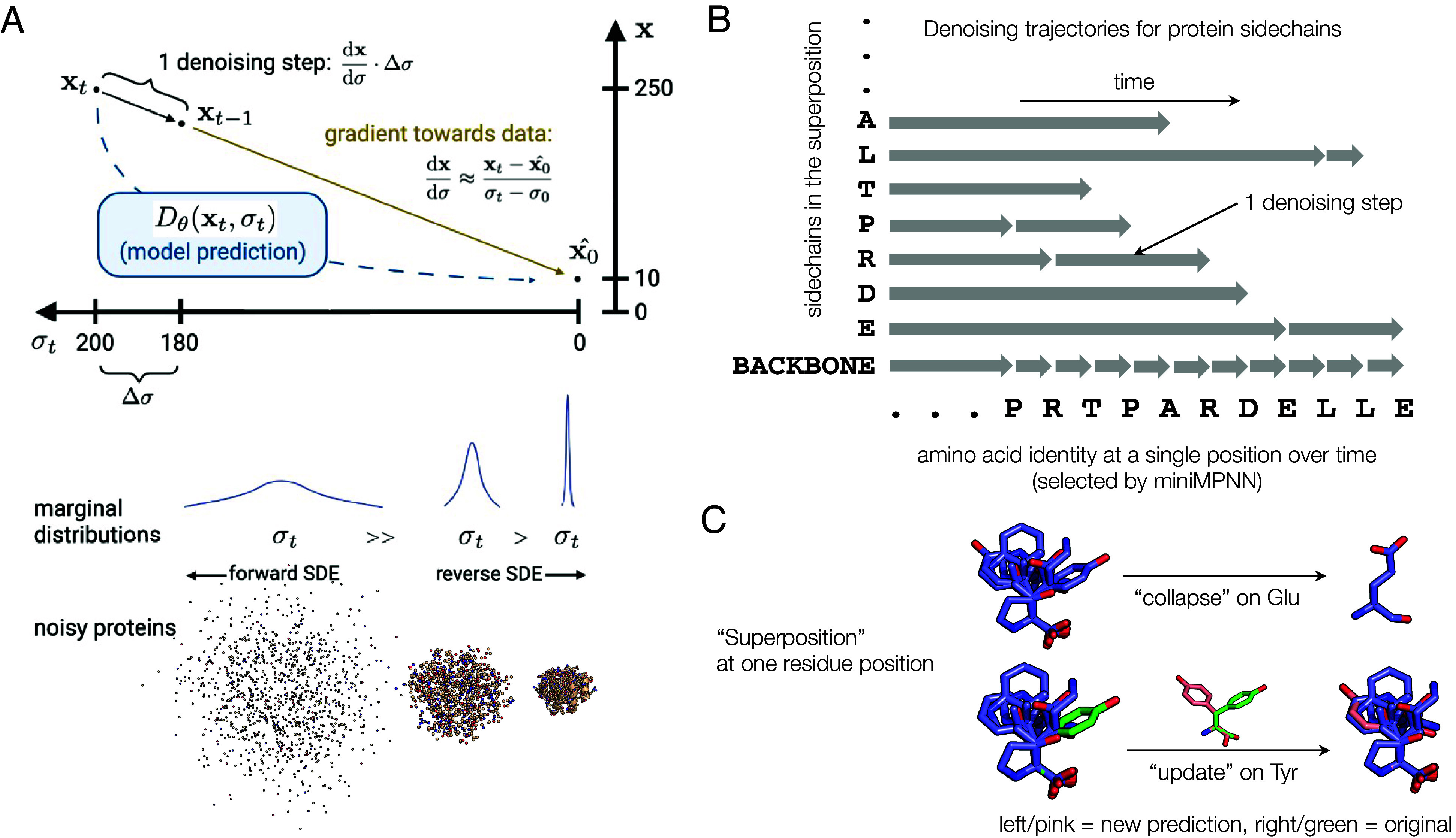
Proteins mediate their functions through chemical interactions; modeling these interactions, which are typically through sidechains, is an important need in protein design. However, constructing an all-atom generative model requires an appropriate scheme for managing the jointly continuous and discrete nature of proteins encoded in the structure and sequence. We describe an all-atom diffusion model of protein structure, Protpardelle, which represents all sidechain states at once as a "superposition" state; superpositions defining a protein are collapsed into individual residue types and conformations during sample generation. When combined with sequence design methods, our model is able to codesign all-atom protein structure and sequence. Generated proteins are of good quality under the typical quality, diversity, and novelty metrics, and sidechains reproduce the chemical features and behavior of natural proteins. Finally, we explore the potential of our model to conduct all-atom protein design and scaffold functional motifs in a backbone- and rotamer-free way.

Keywords: full-atom model; generative modeling; protein design; protein structure; sidechain generation.

Fig. 1.

Superposition modeling approach and denoising scheme for Protpardelle. (A) The basic idea of denoising protein structures by integrating an ODE. Given noisy data ${\mathbf{x}}_t$, we can run the denoising network to predict the fully denoised data, ${\mathbf{x}}_0$. Given the quantities ${\mathbf{x}}_t$, ${\mathbf{x}}_0$, and the noise level ${\sigma }_t$, we can estimate the score, or gradient which points in the direction of data. We can then take a denoising step (integrating the ODE) by choosing a step size $\mathrm{\Delta }\sigma$ and computing an update $\mathrm{\Delta }\mathbf{x}$ on ${\mathbf{x}}_t$ which yields slightly denoised data ${\mathbf{x}}_{t-1}$. We can repeat this many times to iteratively denoise our sample and produce protein samples. The noising process is defined by the marginal distributions, which noise protein structures by simply adding Gaussian noise to the atom coordinates. The scale of these Gaussians increases linearly with time, which induces mostly linear ODE solution trajectories. In our model, the forward noise process acts only on real proteins (with one sidechain per amino acid), whereas the reverse denoising process acts on the full superposition over all possible sidechains. (B) A visualization of the Protpardelle sampling routine for a single residue position. The vertical axis lists the structural elements being denoised (i.e., the atoms of the 20 sidechains in the superposition, plus the backbone atoms). The horizontal axis denotes progression in sampling time, with each amino acid denoting the amino acid predicted for this position at a given timestep. Note that this amino acid prediction can change from step to step. Briefly, at each timestep, we use the predicted amino acid to collapse the superposition and form a “real” but noisy protein, predict denoised positions for each of the atoms in this protein, and then take a denoising step for selected atoms. The size of the denoising step for each atom or sidechain is determined by the last time that atom or sidechain took a denoising step. Each amino acid sidechain from the superposition is denoised only when it is selected by the sequence model. This means that the size of the denoising/integration step varies depending on how frequently that amino acid is predicted. The backbone is denoised at every step since these atoms are common to all amino acids. For more details and the actual sampling algorithm, see Method and Algorithm 1. (C) An example visualization of the sidechain superposition idea and how it might be collapsed or updated, functions which at each denoising step. Sidechains for all 20 amino acids are modeled at once, shown here aligned on the N, CA, and C atoms for a single residue position. Given an amino acid type, we can collapse the superposition from all states to a single state, which yields a “valid” residue or protein. Alternatively, given an amino acid type and newly predicted coordinates for that sidechain, we can update the superposition with new information.

Fig. 2.

Evaluation of proteins sampled from the backbone-only model. (A) Self-consistency performance. We show the RMSD $=$ 2 threshold (dashed line) and the proportion of samples passing this threshold, smoothed with a sliding window of size 21 (solid line). Eight backbones were sampled for each length from 50 to 512. For each backbone, the best of 8 ProteinMPNN-designed sequences is selected and ESMFold is used for all structure predictions. (B) The same samples and ESMFold predictions as in (A), but using the scTM metric. TM is computed using the same alignment as for RMSD. The dashed line indicates TM $=$ 0.5; the solid line indicates proportion of samples with TM $>$ 0.5, smoothed with sliding window of size 11. (C) Example high-quality, novel backbone model samples in green, shown aligned to the ESMFold prediction (blue) and the nearest neighbor in the dataset (red). The lengths, scRMSD, pLDDT, and nnTM metrics for each sample are also shown. (D) The mean over all pairwise TM scores is plotted for all samples (threshold $=$ 0.0), and samples filtered to those with scTM greater than the indicated threshold. Lower values indicate more diversity. (E) Secondary structure content of samples, computed by DSSP. (F) Nearest neighbor distances for model samples with scRMSD $<$ 5. The nnTM is the TM score against the dataset member with the highest TM score to the sample.

Fig. 3.

Evaluation of proteins sampled from the all-atom model trained on CATH + AFDB. (A) Self-consistency performance computed as in Fig. 2, but for the all-atom model. Eight proteins were sampled for each length from 50 to 400. Each protein’s sequence is used for ESMFold, i.e., only one sequence is predicted for each sample, rather than the eight sequences per sample that were predicted for the backbone-only model samples. The success proportion line is smoothed with a sliding window of 21. (B) The same samples and ESMFold predictions as in (A), but using the scTM metric. (C) Example high-quality, novel all-atom model samples. (D) The mean over all pairwise TM scores is plotted for all samples (threshold $=$ 0.0), and samples filtered to those with scTM greater than the indicated threshold. Lower values indicate more diversity. (E) Secondary structure content of samples, computed by DSSP. (F) Nearest neighbor distances for model samples with scRMSD $<$ 5. The nnTM is the TM score against the CATH training set member with the highest TM score to the sample.

Fig. 4.

Analysis of generated all-atom structures, including sidechains. (A–C) Comparison of distributions of (A) bond lengths, (B) bond angles, and (C) chi angles for training data and model samples. Quantities for real data are computed from 100 random proteins from the training set; quantities for model samples are computed from 1 sample for each even-numbered protein length from 50 to 256. These results are computed on samples from an older checkpoint trained on CATH only, but the same chemical quality results hold for newer checkpoints including those trained on AFDB. (D) Detailed views of all-atom raw model output with sidechains built. The bond length RMSE is shown, which is computed by averaging the RMSE between each individual bond length and an idealized bond length in angstroms. For comparison, unrelaxed structures of natural proteins typically have an average bond length RMSE of 0.01 to 0.02. (E) Distribution of fa_dun energies for model samples and natural proteins. Statistics are computed from 5,000 residues chosen at random (without regard to individual proteins) each from the dataset and the set of model samples. The fa_dun energy is computed from the probability of a rotamer given the backbone torsions and a potential term for deviation from an ideal chi angle value. (F) Visualizing the model samples data from (E) on a Ramachandran plot. Each point is a pair of residue backbone torsions, colored by the fa_dun Rosetta energy.

Fig. 5.

Towards all-atom protein design. (A) Performance of unconditional models (trained on CATH or CATH+AFDB) and a crop-conditional model trained on CATH on an augmented version of the RFdiffusion scaffolding benchmark. Left: scaffolding on all atoms of the motif. Right: scaffolding only the ends of fixed sidechains; the atoms after the final rotatable bond. For each model we sample with 40 steps of annealed MCMC and reconstruction guidance. We draw 32 samples for each task and report the success and weak-success rates. Successes are defined as all-atom motif RMSD $<$ 2, backbone motif RMSD $<$ 1, scRMSD $<$ 2, and pLDDT $>$ 70. Weak successes are defined as all-atom motif RMSD $<$ 4, backbone motif RMSD $<$ 3, scTM $>$ 0.5. (B) Example successful all-atom scaffolding designs. (C and D) Potential applications of our model for new approaches to protein design. The conditioning portion is shown in gold on the model sample (green indicates the model-generated portion). These designs are generated with an initial crop-conditional model and reconstruction guidance. (C) An example design generated by scaffolding a TGF-$\beta$1 binding loop including its sidechains. The original binder design (in gold) is a de novo designed monobody and thus is guaranteed not to be in the training set. The pink and cyan chains are TGF-$\beta$1 (PDB: 4KV5). (D) An example design generated by scaffolding only the functional groups of iron-binding Glu and His residues. The model is given only the atoms after the last chi angle: (CG, CD, OE1, OE2) for the Glu residues and (CB, CG, CD2, CE1, ND1, NE2) for the His residues. The native fold shown is chain A of 1BCF.

References

1. Huang P. S., Boyken S. E., Baker D., The coming of age of de novo protein design. Nature 537, 320–327 (2016). - PubMed
1. Korendovych I. V., DeGrado W. F., De novo protein design, a retrospective. Q. Rev. Biophys. 53, e3 (2020). - PMC - PubMed
1. Huang P. S., et al. , Rosettaremodel: A generalized framework for flexible backbone protein design. PLoS ONE 6, e24109 (2011). - PMC - PubMed
1. N. Anand, P. Huang, “Generative modeling for protein structures” in Advances in Neural Information Processing Systems, S. Bengio et al., Eds. (Curran Associates, Inc., 2018), vol. 31, (2018).
1. N. Anand, R. Eguchi, P. S. Huang, Fully differentiable full-atom protein backbone generation. ICLR 2019 Workshop DeepGenStruct (2019). https://openreview.net/forum?id=SJxnVL8YOV. Accessed 6 June 2024.
LinkOut - more resources