Mixed Representations of Sound and Action in the Auditory Midbrain

Abstract

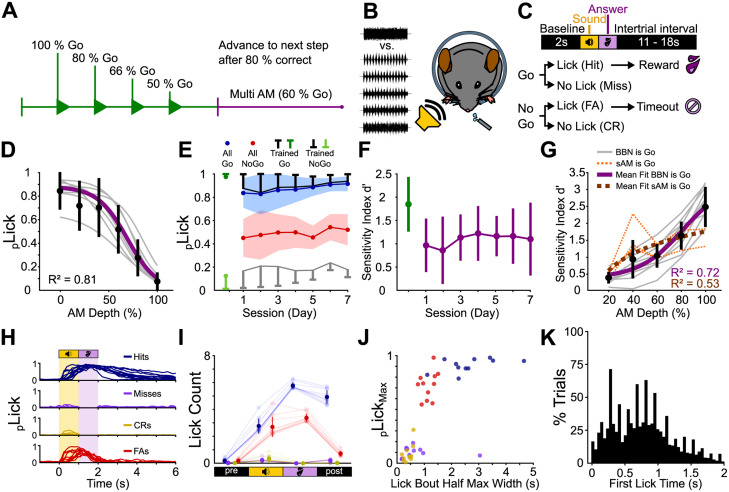
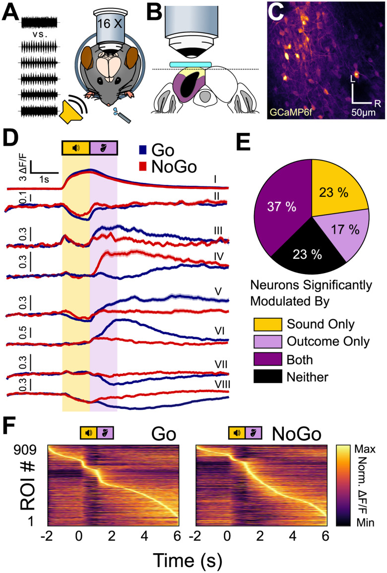
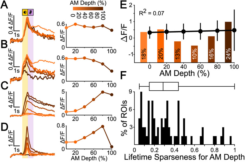
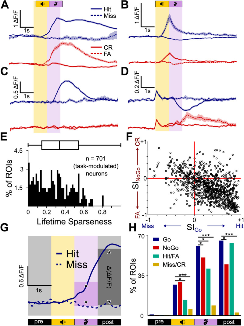
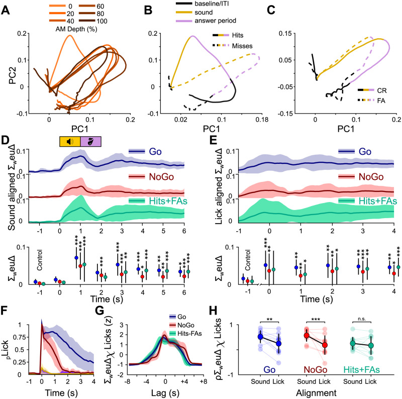
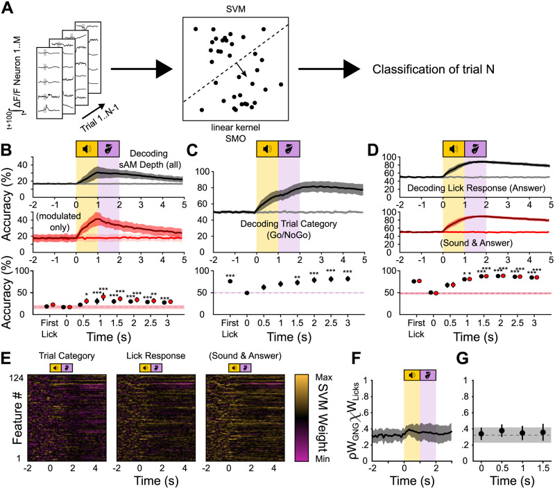
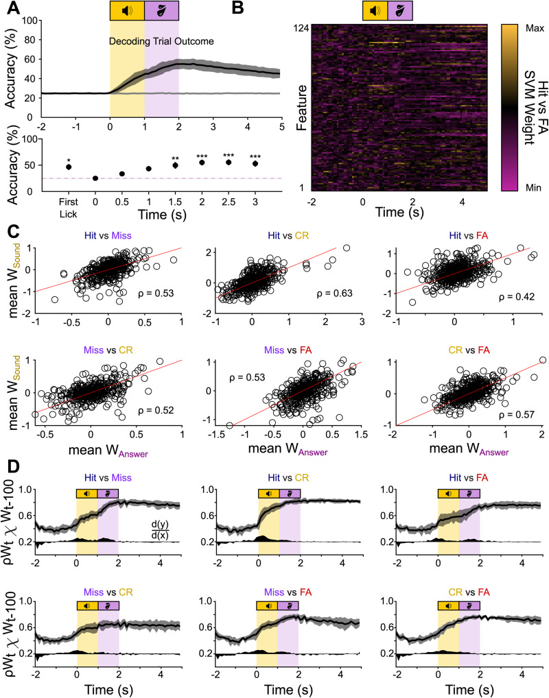
Linking sensory input and its consequences is a fundamental brain operation. During behavior, the neural activity of neocortical and limbic systems often reflects dynamic combinations of sensory and task-dependent variables, and these "mixed representations" are suggested to be important for perception, learning, and plasticity. However, the extent to which such integrative computations might occur outside of the forebrain is less clear. Here, we conduct cellular-resolution two-photon Ca²⁺ imaging in the superficial "shell" layers of the inferior colliculus (IC), as head-fixed mice of either sex perform a reward-based psychometric auditory task. We find that the activity of individual shell IC neurons jointly reflects auditory cues, mice's actions, and behavioral trial outcomes, such that trajectories of neural population activity diverge depending on mice's behavioral choice. Consequently, simple classifier models trained on shell IC neuron activity can predict trial-by-trial outcomes, even when training data are restricted to neural activity occurring prior to mice's instrumental actions. Thus, in behaving mice, auditory midbrain neurons transmit a population code that reflects a joint representation of sound, actions, and task-dependent variables.

Keywords: calcium imaging; inferior colliculus; mixed selectivity; mouse; population analysis.

Figure 1.

Mice discriminate sAM noise from unmodulated noise in a modulation depth-dependent manner. A, Experiment structure. Head-fixed mice were trained to discriminate between 0 and 100% sAM depth (green). We progressively reduced the ratio of Go to No-Go trials as mice's task performance increased until mice reached the multi-sAM stage (purple). B, Upon reaching the criterion (see Results), mice engaged in a “multi-sAM depth” version of the task where the modulation depth of the No-Go sound was varied on a trial-by-trial basis. C, Trial structure. After a 2 s baseline, a sound was presented for 1 s. Licking a waterspout during a 1 s answer period following sound offset was rewarded with a drop of sugar water on Go trials and punished with a 5 s time-out on No-Go trials. Licking at any other point during the trial had no consequence. FA, false alarm; CR, correct rejection. D, Fitted lick probability during the answer period as a function of sAM depth for all mice during multi-sAM sessions. The gray lines are the individual mice, the black circles and lines are the mean ± standard deviation of each sAM depth, and the purple line is the mean fit. E, Mean ± standard deviation lick probability over the final training session (green) and 7 d of multi-sAM sessions for all Go stimuli (blue), all No-Go stimuli (red), and only the trained Go (black) and trained No-Go stimuli (gray). F, d′ for all mice plotted over time for the final training session (Day 0, green) and the 7 d of multi-sAM sessions (purple) as mean ± standard deviation. G, d′ per sAM depth. The gray lines are mice trained on the task contingency described in panels A–F, with BBN employed as the Go sound cue. The dashed orange lines show n = 3 mice that were trained on an opposite contingency with sAM noise as the Go sound cue. The black circles and lines are mean ± standard deviation for each sAM depth, and the purple line is the mean sigmoid fit to “BBN is Go” mice. The dashed dark orange line is the mean logarithmic fit to “sAM is Go” mouse data only. H, Individual average lick histograms for each mouse for all trial outcomes. I, Summary lick statistics for baseline, sound, answer, and intertrial interval periods (1 s each). J, Average maximal lick probability plotted against the full-width at half-maximum of lick bouts, for each mouse and trial category. The outlier miss data point originates from a mouse that routinely licked at low frequency after the end of the response window. K, Histogram of first-lick times for all trials with licks during sound or answer period (n = 3,613 trials).

Figure 2.

Shell IC neurons are active across the entirety of Go and No-Go trials. A, Experimental approach: multiphoton Ca²⁺ imaging was conducted in the superficial shell IC layers to record neural activity as mice engaged in the multi-sAM task. B, Schematic of the imaging plane. A window (teal) was placed above the left IC. The imaging plane was 20–50 µm below the brain surface to reliably target the dorsal shell IC (yellow), rather than the lateral shell (purple) or central IC (black). C, Example field of view from a typical session (L, lateral; R, rostral). D, Example mean ± SEM fluorescence traces of eight separate ROIs on Go (blue) and No-Go (red) trials. All ROIs were recorded simultaneously in the same FOV. Of note is that differential neural activity on Go and No-Go trials spans across the entire trial epoch and is expressed as both increases and decreases in fluorescence. E, The proportion of cells significantly modulated by any sound or outcome, any combination of sound and outcome, or none of those three options (n = 909). F, Normalized mean activity on Go (left) and No-Go (right) trials for all recorded ROIs across all mice's first multi-sAM session, sorted by activity maxima. Of note, most ROIs have their activity maxima after the sound termination.

Figure 3.

Most shell IC neurons are broadly responsive to sAM depth. A, Example ΔF/F traces (left) and sAM depth tuning curve (right) for a broadly tuned representative example cell. B, The same as in A for a cell tuned to high sAM depths. C, The same as in A for a cell tuned to low sAM depths. D, The same as in A for a cell tuned to intermediate sAM depths. E, Mean ± standard deviation of ΔF/F peak for all sound-excited cells (272) shows no linear correlation with sAM depth. The histogram bars indicate the relative proportion of significantly responsive neurons at each sAM depth as determined by trial-to-trial correlation bootstrapping analysis. F, Lifetime sparseness for sAM depth responses of all neurons with significant activity during sound presentation.

Figure 4.

Trial outcome selectivity of individual Shell IC neurons. A, Mean ± SEM ΔF/F traces of an example neuron selective for hit and false alarm (FA) trial outcomes. B–D, Same as in A, but for a neuron responding on misses and correct rejections (CR; B), hits only (C), and with opposing activity on hits and false alarms (D). E, Lifetime sparseness for outcome responses of all 701 significantly task-modulated neurons. F, Selectivity Indices on Go and No-Go trials are plotted for each neuron on the x- and y-axes, respectively. G, Schematic of the Δ(ΔF/F) analysis. The mean ΔF/F in 1 s bins was computed on a trial-by-trial basis for each neuron and compared across trial outcomes using a Wilcoxon rank sum test. H, The proportion of neurons with significantly different ΔF/F values for (from left to right) hits and misses (blue), correct rejections and false alarms (red), hits and false alarms (green), and misses and correct rejections (orange) per averaging period. *p < 0.05; **p < 0.01; ***p < 0.001.

Figure 5.

Population dynamics revealed through principal component analysis show trial outcome–dependent differences. A, Example PCA-based trajectory from a single mouse sorted by AM depth. For visualization purposes, only the first two components are displayed, collectively explaining ∼80% of the total variance. B, The same example sorted by trial outcome for Go trials (hits/misses). Of note, the trajectories for hits and misses start to diverge immediately after the baseline. C, The same as in B but for No-Go trials. D, Top, The sum of weighted Euclidean distances over all principal components over time for hits/misses (blue), correct rejections/false alarms (red), and hits/false alarms (FA, green) aligned to sound onset for all mice and sessions, plotted as mean and standard deviation. Bottom, Friedman's test followed by a Dunnett's post hoc test comparing the mean sum of weighted Euclidean distances against the baseline at t = −1 s. E, The same as in D, but the data were aligned to the first lick after sound onset prior to computing the PCA. F, Average lick histograms sorted by trial outcome for the initial multi-sAM session for all mice, given as mean and standard deviation and aligned to the first sound-evoked lick. G, The mean and standard deviation z-scored cross-correlation functions for sound-aligned ΔF/F traces and lick histograms for Go (blue), No-Go (red), and hit/false alarm trials (green). H, Pearson’s correlation coefficient distributions of ΔF/F traces and lick histograms for Go (blue), No-Go (red), and hit/false alarm trials (green) for sound-aligned data and lick-aligned data. Statistics are two-sample Wilcoxon signed rank tests. *p < 0.05; **p < 0.01; ***p < 0.001.

Figure 6.

An SVM classifier can predict task-related variables from the neural activity before, during, and after mice's instrumental actions. A, Schematic of the SVM classifier. Training data is the integral of the ΔF/F traces of all neurons in a 100 ms sliding window across the trial. Accuracy is plotted over the beginning of the integration time. B, Top, Classification accuracy over time for a decoder trained to classify sAM depth. The raw accuracy was normalized to obtain the balanced accuracy (black trace) and balanced shuffled accuracy (gray trace), normalizing the chance level to 16.67% (1 divided by the number of classes; see Materials and Methods). Middle, The same as in top but only using modulated stimuli (sAM depths 20–100%). Bottom, Friedman’s test with Dunnett's post hoc comparisons for each 0.5 s time bin against the baseline accuracy at −1 s (dashed line) for all sAM depth trials (black) or only modulated trials (red). Data points labeled “first lick” are classifiers trained on fluorescence data limited to before mice's first lick after sound onset on each trial. C, Same as in B but for the trial category. The chance level is normalized to 50% (see Materials and Methods). D, Top, Same as in B but for lick response during the answer period. The chance level is normalized to 50% (see Materials and Methods). Middle, The same as in top, but for lick response during the sound or answer period. Bottom, Friedman’s test with Dunnett's post hoc test comparing time points against the baseline accuracy at −1 s for top data (black) and the middle data (red). E, Examples of SVM feature (ROI) weights over time for a binary classifier distinguishing Go from No-Go trials (left), lick from no-lick trials determined by the answer (middle) and sound or answer period (right). F, Mean correlation coefficients for the feature weights of the “trial category” and “lick response” decoders from C and D (top). Each point in time represents the mean and standard deviation of Pearson’s coefficients for two matched individual columns from E (feature weights at a single time point). G, Statistics from F, Friedman's test with Dunnett's post hoc test against baseline (t = −1 s). *p < 0.05; **p < 0.01; ***p < 0.001.

Figure 7.

The outcome classifier uses overlapping information during the sound- and the outcome period. A, Top, Classification accuracy over time for a decoder trained to classify trial outcome. The raw accuracy was normalized to obtain the balanced accuracy (black trace) and balanced shuffled accuracy (gray trace), normalizing the chance level to 25% (1 divided by the number of classes; see Materials and Methods). Bottom, Friedman’s test with Dunnett's post hoc test comparing time points against the baseline accuracy at −1 s. B, An example set of weights for a binary classifier (hit/false alarm) of the set of subclassifiers that make up the outcome classifier. C, Mean feature weights during the sound (y-axis) and answer period (x-axis) for all ROIs for the subclassifiers distinguishing hits and misses, hits and correct rejections (CR), hits and false alarms (FA), misses and correct rejections, misses and false alarms, and correct rejections and false alarms. The red lines are unity lines. D, Mean correlation coefficients for the feature weights of the subclassifiers at time t and time t − 100 ms. The black area below the curve indicates the first derivative to visualize the steps of increased correlation in arbitrary units, with d(y)/d(x) = 0 at 0.2 on the y-axis. *p < 0.05; **p < 0.01; ***p < 0.001.

References

1. Aitkin LM, Kenyon CE, Philpott P (1981) The representation of the auditory and somatosensory systems in the external nucleus of the cat inferior colliculus. J Comp Neurol 196:25–40. 10.1002/cne.901960104 - DOI - PubMed
1. Aitkin LM, Phillips SC (1984) Is the inferior colliculus and obligatory relay in the cat auditory system? Neurosci Lett 44:259–264. 10.1016/0304-3940(84)90032-6 - DOI - PubMed
1. Audette NJ, Schneider DM (2023) Stimulus-specific prediction error neurons in mouse auditory cortex. J Neurosci 43:7119–7129. 10.1523/JNEUROSCI.0512-23.2023 - DOI - PMC - PubMed
1. Bajo VM, Nodal FR, Bizley JK, Moore DR, King AJ (2007) The ferret auditory cortex: descending projections to the inferior colliculus. Cereb Cortex 17:475–491. 10.1093/cercor/bhj164 - DOI - PMC - PubMed
1. Bajo VM, Nodal FR, Moore DR, King AJ (2010) The descending corticocollicular pathway mediates learning-induced auditory plasticity. Nat Neurosci 13:253–260. 10.1038/nn.2466 - DOI - PMC - PubMed
LinkOut - more resources