Spatial mapping of mobile genetic elements and their bacterial hosts in complex microbiomes

Abstract

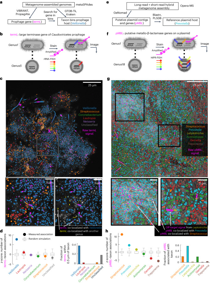
The exchange of mobile genetic elements (MGEs) facilitates the spread of functional traits including antimicrobial resistance within bacterial communities. Tools to spatially map MGEs and identify their bacterial hosts in complex microbial communities are currently lacking, limiting our understanding of this process. Here we combined single-molecule DNA fluorescence in situ hybridization (FISH) with multiplexed ribosomal RNA-FISH to enable simultaneous visualization of both MGEs and bacterial taxa. We spatially mapped bacteriophage and antimicrobial resistance (AMR) plasmids and identified their host taxa in human oral biofilms. This revealed distinct clusters of AMR plasmids and prophage, coinciding with densely packed regions of host bacteria. Our data suggest spatial heterogeneity in bacterial taxa results in heterogeneous MGE distribution within the community, with MGE clusters resulting from horizontal gene transfer hotspots or expansion of MGE-carrying strains. Our approach can help advance the study of AMR and phage ecology in biofilms.

Fig. 1. Single-molecule MGE-FISH.

a, Diagram of E. coli model GFP plasmid system used to optimize single-molecule FISH. b, (i) Diagrams of different methods implemented. Blue cells on the left are wild type and orange cells on the right are transformed with the plasmid. After the first row, two encoding probes are shown to represent ten encoding probes in all cases. Magenta lines represent the plasmid, cyan represents 16S rRNA and blue represents off-target binding sites. (ii) Representative images for each method alteration. Magenta indicates a signal from MGE-FISH and cyan indicates a signal from 16S rRNA-FISH. Scale bar, 5 µm. Images were captured for at least 1,000 cells in each condition. (iii) Fraction of cells with spots for control and plasmid images as a function of signal-to-noise ratio (SNR) threshold. SNR was calculated for each spot, dividing the spot signal by the average background signal (‘Manual spot background filtering’ in Methods). Black vertical line indicates the selected SNR threshold. TPR, true positive rate; FPR, false positive rate (at the threshold). (iv) Histograms for the number of spots in each cell. Width indicates the frequency of the spot count value. Horizontal red bars indicate mean spot count. c, Left: diagram of MGE-FISH staining of E. coli infected by T4 phage. Middle: example images for four multiplicities of infection at 20 min and 30 min after introducing phage to the culture. Right: results of manual counting to classify cells into groups on the basis of the number of MGE-FISH spots.

Fig. 2. MGE-FISH in human oral plaque.

a, Diagram of the workflow to apply MGE-FISH in oral plaque biofilms (created with BioRender.com). b, Left: example images of plaque, transformed E. coli expressing GFP, and the combination of both plaque and E. coli. All samples were stained for the GFP gene using MGE-FISH. The experiment was repeated three times with similar results. Right: association of MGE-FISH signal with GFP cells and non-GFP cells in each sample. c, Left: diagram of two-volunteer control experiment. Middle: example images of plaque samples from each volunteer stained for the mefE gene. At least three tiled fields of view (FOVs) were collected for each sample with similar results. Right: measurement of relative spot count for each volunteer. Spot counts for each image were normalized by dividing the number of segmented spots by the number of segmented cells (‘Semi-automated image segmentation’ in Methods). d, Top left: diagram showing the multicolour approach used to stain the gene termL. Bottom left: example FOV plotted as separate density maps for each colour of termL probes. At least three tiled FOVs were collected for each sample with similar results. Inset 1: zoomed region of the plaque overlaid with all colours of termL stain. Inset 2: zoomed region of plaque split into each colour of termL probes. Right: measurements of termL colour co-localization normalized as the fraction of total spots. e, Top left: diagram showing the multicolour approach used to simultaneously stain the genes patA, patB and adeF. Bottom left: example FOV plotted as separate density maps for each gene. At least three tiled FOVs were collected for each sample with similar results. Inset 1: zoomed region of the plaque overlaid with all colours. Inset 2: zoomed region of plaque split by gene. Right: measurement of co-localization of patB spots with each other gene normalized as the fraction of patB spots co-localized.

Fig. 3. Combined MGE and taxonomic mapping.

a, Workflow for prophage host association predictions via metagenomic sequencing assembly, binning and phage gene prediction. b, Diagram showing simultaneous single-colour rRNA stain for taxon mapping and HCR staining for prophage mapping. c, Top: bacterial genera classified by rRNA-FISH overlaid with the raw signal from MGE-FISH on termL prophage gene. Bottom left: zoomed region of rRNA-FISH overlaid with MGE-FISH. Bottom right: zoomed region showing only Veillonella (blue) and termL (magenta and yellow) in colour, while all other cells are greyscale. The arrows indicate examples of termL signal co-localized with Veillonella in magenta and termL signal co-localized with another genus in yellow. d, Left: z-scores for the number of associations between termL and each genus (circles) compared to simulation where the termL spots are randomly assigned to cells (boxplots, 1,000 simulations). The bounds of the boxes show the first quartile to the third quartile, the centre shows the median and the whiskers show the farthest data point lying within 1.5× the IQR. Right: fraction of termL spots associated with each taxon. Association between a cell and a spot is defined as the nearest neighbour cell to the spot. e, Workflow for plasmid host association prediction via metagenomic sequencing assembly, plasmid prediction and alignment to a reference database. f, Diagram showing simultaneous multicolour HiPR-FISH rRNA staining for taxon mapping and HCR staining for plasmid mapping. g, Top: bacterial genera classified by HiPR-FISH overlaid with raw signal from MGE-FISH on pMBL genes. Bottom: two zoomed regions of HiPR-FISH overlayed with MGE-FISH. For all MGE-FISH spot association measurements, we filtered large non-circular signal as shown at the bottom right in Leptotrichia cells. h, Left: z-scores for the number of associations between pMBL and each genus (circles) compared to simulation where the pMBL spots are randomly assigned to cells (boxplots, 1,000 simulations). The bounds of the boxes show the first quartile to the third quartile, the centre shows the median and the whiskers show the farthest data point lying within 1.5× the IQR. Right: fraction of pMBL spots associated with each taxon. Association between a cell and a spot is defined as the nearest neighbour cell to the spot.

Fig. 4. Identifying the host taxon of a previously undescribed plasmid.

a, Diagram illustrating sample collection from a patient with stage 3 periodontitis followed by DNA extraction for long-read Nanopore sequencing and short-read Illumina sequencing (created with BioRender.com). The same sample was then used for simultaneous HiPR-FISH and MGE-FISH staining. b, Diagram of a plasmid assembled from long- and short-read sequencing. The inner axes plot Illumina short-read alignment as reads per base and the middle axes do the same for Nanopore long reads. The outer bars plot the locations and names of predicted genes, where arrows and ‘+/−’ at the start of the names indicate gene orientation. Pink bars indicate the locations of encoding probes for HCR staining, while light grey bars indicate the locations of non-fluorescently stained helper probes. c, Bacterial genera classified by HiPR-FISH overlaid with the raw signal from MGE-FISH on the previously undescribed plasmid. Grey indicates the raw signal from autofluorescence in unstained sample material. d, Left: z-scores for the number of associations between the plasmid and each genus (circles) compared to simulation of random distributions of the same spots (boxplots, 1,000 simulations). The bounds of the boxes show the first quartile to the third quartile, the centre shows the median and the whiskers show the farthest data point lying within 1.5× the IQR. Right: fraction of plasmid spots associated with each genus.

Extended Data Fig. 1. In vitro single MGE-FISH on plasmids and phage.

a Subcellular spot locations MGE-FISH staining of GFP-plasmid normalized to average cell shape plotted as spot density. The colormap is nonlinear and maps to values using a power law where color value x maps to density value y = x^2.5. b Example zoomed raw images of cells where spots are located at the poles. c Example images of MGE-FISH staining of T4 phage gp34 gene in T4 phage infection time series. Cyan: 16S rRNA, magenta: GFP DNA. d Example cells showing examples for the different classification of cells in the manual counting data in Fig. 1c.

Extended Data Fig. 2. Evaluation of MGE-FISH in plaque biofilms.

a Visualization of cell segmentation and spot counting on a zoom region (gray box on the left) of Fig. 2c. Green outlines in top right image indicate cell segmentations and green dots on the bottom right image indicate spot locations. b Spatial autocorrelation of mefE spots using Moran’s I statistic. Colored vertical bar indicates the observed value, black vertical bar indicates the mean value of the simulation, and the shaded area indicates the histogram of the simulation. For the simulation spots were randomly redistributed on the same set of cell segmentations 1000 times. The Monte Carlo method with 1000 simulations was used in a two-sided test to evaluate the null hypotheses of random distribution of spots. c Top: diagram of orthogonal control probes that should produce no signal. Bottom: diagram of the gel embedding, nucleic acid anchoring, and sample clearing process. d Left: Example images showing the off-target signal from orthogonal probes in uncleared and cleared plaque samples. At least three tiled fields of view were collected for each sample with similar results. Center: spot counts normalized by number of cells as a function of signal to noise ratio (SNR). Right: Measurement of non-spot pixels normalized by cell pixels.

Extended Data Fig. 3. Control experiments for T7-like prophage capsB minor capsid protein in Plaque.

a Top left: example images showing regions of cells with similar morphology cells. From right to left the images are: MGE-FISH controls with no encoding probes, encoding probes that are orthogonal as determined by metagenomic analysis, or probes targeting capsB. Top right: spot counts from each control normalized by number of cells. Bottom: observed Moran’s I spatial autocorrelation values (vertical black lines) compared to 999 simulations of random spot distribution (filled curves). The Monte Carlo method with 999 simulations was used in a two-sided test to evaluate the null hypotheses of random distribution of spots. P-values were 0.40, 0.38, and <0.01 for images captured using no encoding probes, orthogonal encoding probes, and capsB encoding probes respectively. b Example FOV showing a large hotspot of prophage (~100μm). Inset square shows the location of the capsB example image in a.

Extended Data Fig. 4. AMR gene distribution measurements.

a Example image showing spatially clustered signal from an AMR gene, pMBL, found on a plasmid in the metagenomic sequencing data. pMBL signal is in magenta and the 16 s rRNA signal is in gray. b Top: Histograms of pMBL nearest neighbor distances for the observed pMBL spots (magenta) in a and 100 simulations of randomly distributed pMBL spots (black). The solid blue line shows the mean of the simulated histograms. 97.5% of simulation values were less than the top dotted blue line, and 97.5% of simulation values were greater than the bottom dotted blue line. The Monte Carlo method with 100 simulations was used in a two-sided test to evaluate the null hypotheses of random distribution of spots. Bottom: Empirical probability that a pMBL spot has a nearest neighbor distance less than the given distance for observed pMBL spots (magenta) and simulated random pMBL spots (black). Blue solid and dashed lines are plotted as above. c Empirical pair correlation function for observed (magenta) and simulated (black) pMBL spots. Values indicate the radial density of pMBL spots at a given distance from a reference spot. Blue solid and dashed lines are plotted as above.

Extended Data Fig. 5. Diagram of the previously undescribed plasmid.

Same as Fig. 4b but with additional information. The second ring from the inside indicates in blue the number of tetramers of G or C nucleotide bases in the assembled sequence per 50 base pair window. The second ring from the outside indicates the GC skew in a 50 bp window where 0 indicates equal counts of G and C bases, positive indicates excess G bases, and negative indicates excess C bases.

References

1. Munita, J. M. & Arias, C. A. in Virulence Mechanisms of Bacterial Pathogens (eds Kudva, I. T. et al.) 481–511 (John Wiley & Sons, 2016).
1. Khan Mirzaei, M. & Deng, L. New technologies for developing phage-based tools to manipulate the human microbiome. Trends Microbiol.30, 131–142 (2022). 10.1016/j.tim.2021.04.007 - DOI - PubMed
1. Rasmussen, T. S. et al. Bacteriophage-mediated manipulation of the gut microbiome – promises and presents limitations. FEMS Microbiol. Rev.44, 507–521 (2020). 10.1093/femsre/fuaa020 - DOI - PubMed
1. Gordillo Altamirano, F. L. & Barr, J. J. Phage therapy in the postantibiotic era. Clin. Microbiol. Rev. 32, e00066-18 (2019). - PMC - PubMed
1. Penders, J., Stobberingh, E., Savelkoul, P. & Wolffs, P. The human microbiome as a reservoir of antimicrobial resistance. Front. Microbiol.4, 87 (2013). 10.3389/fmicb.2013.00087 - DOI - PMC - PubMed
MeSH terms
LinkOut - more resources