Lightning Pose: improved animal pose estimation via semi-supervised learning, Bayesian ensembling and cloud-native open-source tools

Abstract

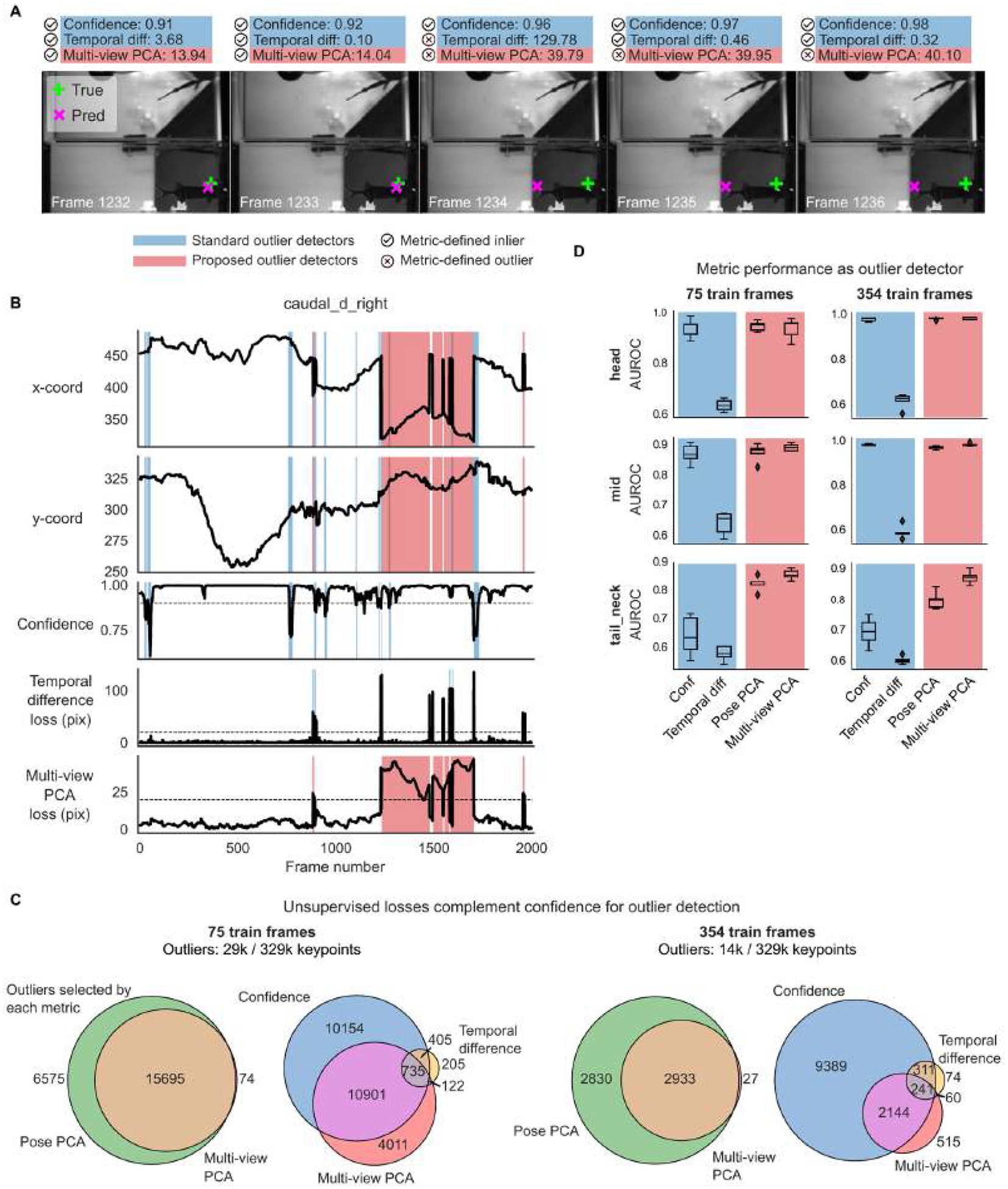
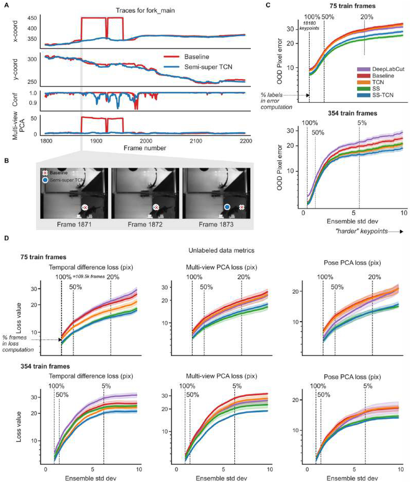
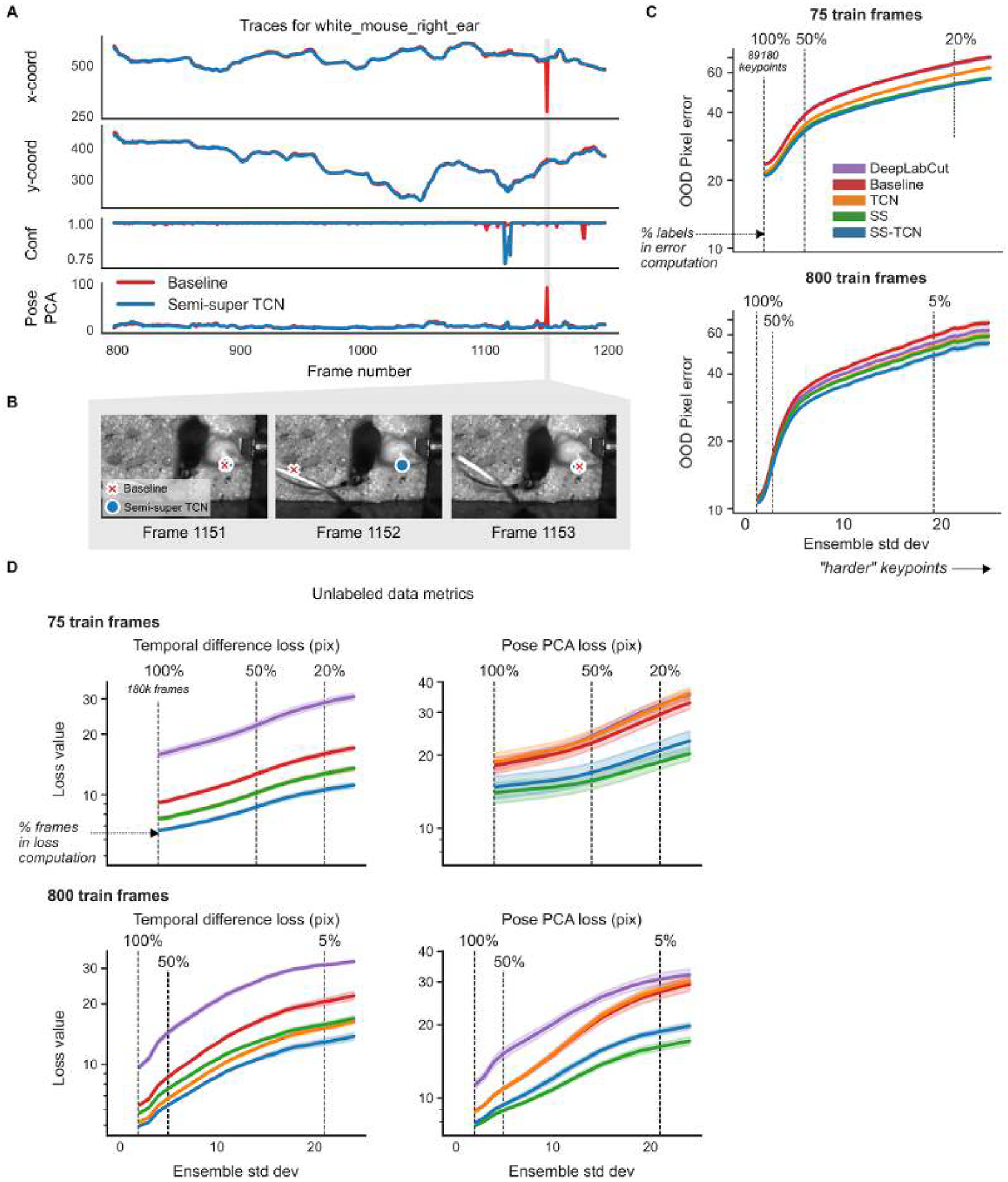
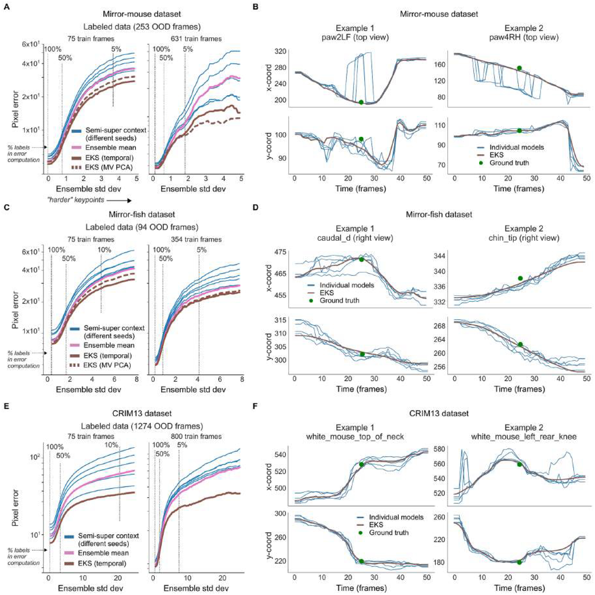
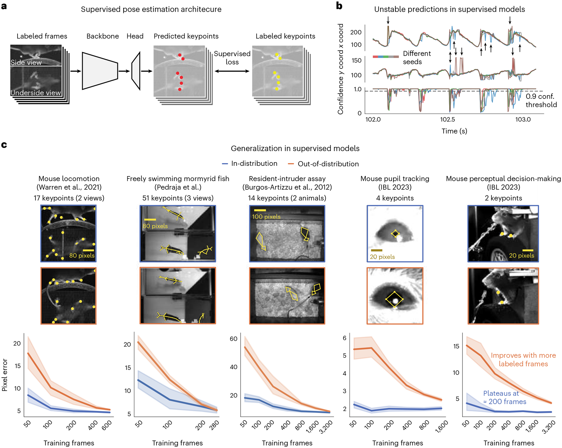
Contemporary pose estimation methods enable precise measurements of behavior via supervised deep learning with hand-labeled video frames. Although effective in many cases, the supervised approach requires extensive labeling and often produces outputs that are unreliable for downstream analyses. Here, we introduce 'Lightning Pose', an efficient pose estimation package with three algorithmic contributions. First, in addition to training on a few labeled video frames, we use many unlabeled videos and penalize the network whenever its predictions violate motion continuity, multiple-view geometry and posture plausibility (semi-supervised learning). Second, we introduce a network architecture that resolves occlusions by predicting pose on any given frame using surrounding unlabeled frames. Third, we refine the pose predictions post hoc by combining ensembling and Kalman smoothing. Together, these components render pose trajectories more accurate and scientifically usable. We released a cloud application that allows users to label data, train networks and process new videos directly from the browser.

Extended Data Fig. 1|. Unsupervised losses complement model confidence for outlier detection on mirror-fish dataset.

Example traces, unsupervised metrics, and predictions from a DeepLabCut model (trained on 354 frames) on held-out videos. Conventions for panels A-D as in Fig. 3. A: Example frame sequence. B: Example traces from the same video. C: Total number of keypoints flagged as outliers by each metric, and their overlap. D: Area under the receiver operating characteristic curve for several body parts. We define a ‘true outlier’ to be frames where the horizontal displacement between top and bottom predictions or the vertical displacement between top and right predictions exceeds 20 pixels. AUROC values are only shown for the three body parts that have corresponding keypoints across all three views included in the Pose PCA computation (many keypoints are excluded from the Pose PCA subspace due to many missing hand labels). AUROC values are computed across frames from 10 test videos; boxplot variability is over n=5 random subsets of training data. The same subset of keypoints is used for panel C. Boxes in panel D use 25th/50th/75th percentiles for min/center/max; whiskers extend to 1.5 * IQR.

Extended Data Fig. 2 |. Unsupervised losses complement model confidence for outlier detection on CRIM13 dataset.

Example traces, unsupervised metrics, and predictions from a DeepLabCut model (trained on 800 frames) on held-out videos. Conventions for panels A-C as in Fig. 3. A: Example frame sequence. B: Example traces from the same video. Because the size of CRIM13 frames are larger than those of the mirror-mouse and mirror-fish datasets, we use a threshold of 50 pixels instead of 20 to define outliers through the unsupervised losses. C: Total number of keypoints flagged as outliers by each metric, and their overlap. Outliers are collected from predictions across frames from 18 test videos and across predictions from five different networks trained on random subsets of labeled data.

Extended Data Fig. 3|. PCA-derived losses drive most improvements in semi-supervised models.

For each model type we train three networks with different random seeds controlling the data presentation order. The models train on 75 labeled frames and unlabeled videos. We plot the mean pixel error and 95% CI across keypoints and OOD frames, as a function of ensemble standard deviation, as in Fig. 4. At the 100% vertical line, n=17150 keypoints for mirror-mouse, n=18180 for mirror-fish, and n=89180 for CRIM13.

Extended Data Fig. 4 |. Unlabeled frames improve pose estimation in mirror-fish dataset.

Conventions as in Fig. 4. A. Example traces from the baseline model and the semi-supervised TCN model (trained with 75 labeled frames) for a single keypoint on a held-out video (Supplementary Video 6). B. A sequence of frames corresponding to the grey shaded region in panel (A). C. Pixel error as a function of ensemble standard devation for scarce (top) and abundant (bottom) labeling regimes. D. Individual unsupervised loss terms plotted as a function of ensemble standard deviation for the scarce (top) and abundant (bottom) label regimes.

Extended Data Fig. 5 |. Unlabeled frames improve pose estimation in CRIM13 dataset.

Conventions as in Fig. 4.A. Example traces from the baseline model and the semi-supervised TCN model (trained with 800 labeled frames) for a single keypoint on a held-out video (Supplementary Video 7). B. A sequence of frames corresponding to the grey shaded region in panel (A). C. Pixel error as a function of ensemble standard deviation for scarce (top) and abundant (bottom) labeling regimes. D. Individual unsupervised loss terms plotted as a function of ensemble standard deviation for the scarce (top) and abundant (bottom) labeling regimes.

Extended Data Fig. 6 ∣. The Ensemble Kalman Smoother improves pose estimation across datasets.

We trained an ensemble of five semi-supervised TCN models on the same training data. The networks differed in the order of data presentation and in the random weight initializations for their ‘head’. This figure complements Fig. 5 which uses an ensemble of DeepLabCut models as input to EKS. A. Mean OOD pixel error over frames and keypoints as a function of ensemble standard deviation (as in Fig. 4). B. Time series of predictions (x and y coordinates on top and bottom, respectively) from the five individual semi-supervised TCN models (75 labeled training frames; blue lines) and EKS-temporal (brown lines). Ground truth labels are shown as green dots. C,D. Identical to A,B but for the mirror-fish dataset. E,F. Identical to A,B but for the CRIM13 dataset.

Extended Data Fig. 7 |. Lightning Pose models and ensemble smoothing improve pose estimation on IBL paw data.

A. Sample frames from each camera view overlaid with a subset of paw markers estimated from DeepLabCut (left), Lightning Pose using a semi-supervised TCN model (center), and a 5-member ensemble using semi-supervised TCN models (right). B. Example left view frames from a subset of 44 IBL sessions. C. The empirical distribution of the right paw position from each view projected onto the 1D subspace of maximal correlation in a canonical correlation analysis (CCA). Column arrangement as in A. D. Correlation in the CCA subspace is computed across n=44 sessions for each model and paw. The LP+EKS model has a correlation of 1.0 by construction. E. Median right paw speed plotted across correct trials aligned to first movement onset of the wheel; error bars show 95% confidence interval across n=273 trials. The same trial consistency metric from Fig. 6 is computed. F. Trial consistency computed across n=44 sessions. G. Example traces of Kalman smoothed right paw speed (blue) and predictions from neural activity (orange) for several trials using cross-validated, regularized linear regression. H. Neural decoding performance across n=44 sessions. Panels D, F, and H use a one-sided Wilcoxon signed-rank test; boxes use 25th/50th/75th percentiles for min/center/max; whiskers extend to 1.5 * IQR. See Supplementary Table 2 for further quantification of boxes.

Extended Data Fig. 8 |. Lightning Pose enables easy model development, fast training, and is accessible via a cloud application.

A. Our software package outsources many tasks to existing tools within the deep learning ecosystem, resulting in a lighter, modular package that is easy to maintain and extend. The innermost purple box indicates the core components: accelerated video reading (via NVIDIA DALI), modular network design, and our general-purpose loss factory. The middle purple box denotes the training and logging operations which we outsource to PyTorch Lightning, and the outermost purple box denotes our use of the Hydra job manager. The right box depicts a rich set of interactive diagnostic metrics which are served via Streamlit and FiftyOne GUIs. B. A diagram of our cloud application. The application’s critical components are dataset curation, parallel model training, interactive performance diagnostics, and parallel prediction of new videos. C. Screenshots from our cloud application. From left to right: LabelStudio GUI for frame labeling, TensorFlow monitoring of training performance overlaying two different networks, FiftyOne GUI for comparing these two networks’ predictions on a video, and a Streamlit application that shows these two networks’ time series of predictions, confidences, and spatiotemporal constraint violations.

Fig. 1|. Fully supervised pose estimation often outputs unstable predictions and requires many labels to generalize to new animals.

a, Diagram of a typical pose estimation model trained with supervised learning, illustrated using the mirror-mouse dataset. A dataset is created by labeling keypoints on a subset of video frames. A convolutional neural network, consisting of a ‘backbone’ and a prediction ‘head’, takes in a batch of frames as inputs, and predicts a set of keypoints for each frame. It is trained to minimize the distance from the labeled keypoints. b, Predictions from five supervised DeepLabCut networks (trained with 631 labeled frames on the mirror-mouse dataset), for the left front paw position (top view) during 1 s of running behavior (Supplementary Video 1). Top, $x$-coordinate; middle, $y$-coordinate; bottom, confidence, applying a standard 0.9 threshold indicated by the dashed line. Black arrows indicate example time points where there is disagreement among the network predictions. c, Top row shows five example datasets. Each blue image is an example taken from the InD test set, which contains new images of animals that were seen in the training set. The orange images are test examples from unseen animals altogether, which we call the OOD test set. Bottom row shows data efficiency curves, measuring test-set pixel error as a function of the training set size. InD pixel error is shown in blue and OOD in orange. Line plots show the mean pixel error across all keypoints and frames ± s.e. over $n=10$ random subsets of InD training data.

Fig. 2 |. Lightning Pose exploits unlabeled data in pose estimation model training.

a, Diagram of the semi-supervised model that contains supervised (top row) and unsupervised (bottom row) components. b, Temporal difference loss. Top left: illustration of a jump discontinuity. Top right: loss landscape for frame t given the prediction at $t-1$ (white diamond), for the left front paw (top view). The dark blue circle corresponds to the maximum allowed jump, below which the loss is set to zero. Bottom left: correlation between temporal difference loss and pixel error on labeled test frames. c, Multi-view PCA loss. Top left: illustration of a 3D keypoint detected on the imaging plane of two cameras. Top right: loss landscape for the left front paw (top view; white diamond) given its predicted location on the bottom view. The blue band of low loss values is an ‘epipolar line’ on which the top-view paw could be located. Bottom left: correlation between multi-view PCA loss and pixel error. Bottom right: cumulative variance explained for single body part labels across all views versus the fraction of principal components (PCs) kept on multi-view datasets. d, Pose PCA loss. Top left: illustration of plausible and implausible poses. Top right: loss landscape for the left front paw (top view; white diamond) given all other keypoints, which is minimized around the paw’s actual position. Bottom left: correlation between Pose PCA loss and pixel error. Bottom right: cumulative variance explained for pose labels versus fraction of PCs kept. e, The TCN processes each labeled frame with its adjacent unlabeled frames, using a bidirectional CRNN. It forms two sets of location heat map predictions, one using single-frame information and another using temporal context.

Fig. 3 |. Unsupervised losses complement model confidence for outlier detection.

a, Example frame sequence from the mirror-mouse dataset. Predictions from a DeepLabCut model (trained on 631 frames) are overlaid (magenta ×), along with the ground truth (green +). Open white circles denote the location of the same body part (left hind paw) in the other (top) view; given the geometry of this setup, a large horizontal displacement between the top and bottom predictions indicates an error. Each frame is accompanied with ‘standard outlier detectors’, including confidence, temporal difference loss (shaded in blue) and ‘proposed outlier detectors’, including multi-view PCA loss (shaded in red; Pose PCA excluded for simplicity), indicates an inlier as defined by each metric, and indicates an outlier. b, Example traces from the same video. Blue background denotes times where standard outlier detection methods flag frames: confidence falls below a threshold (0.9) and/or the temporal difference loss exceeds a threshold (20 pixels). Red background indicates times where the multi-view PCA error exceeds a threshold (20 pixels). Purple background indicates both conditions are met. c, The total number of keypoints flagged as outliers by each metric, and their overlap. d, AUROC for each paw, for DeepLabCut models trained with 75 and 631 labeled frames (left and right columns, respectively). AUROC = 1 indicates the metric perfectly identifies all nominal outliers in the video data; 0.5 indicates random guessing. AUROC values are computed across all frames from 20 test videos; box plot variability is over $n=5$ random subsets of training data. Boxes use the 25th, 50th and 75th percentiles for minimum, center and maximum values, respectively; whiskers extend to 1.5 times the interquartile range (IQR).

Fig. 4 |. Unlabeled frames improve pose estimation (raw network predictions).

a, Example traces from the baseline model and the semi-supervised TCN model (trained with 75 labeled frames) for a single keypoint (right hind paw; top view) on a held-out video (Supplementary Video 5). One erroneous paw switch is shaded in gray. b, A sequence of frames (1,548–1,551) corresponding to the gray shaded region in a in which a paw switch occurs. c, We computed the standard deviation of each keypoint prediction in each frame in the OOD labeled data across all model types and seeds (five random shuffles of training data). We then took the mean pixel error over all keypoints with a standard deviation larger than a threshold value, for each model type. Smaller standard deviation thresholds include more of the data ($n=\mathrm{17,150}$ keypoints total, indicated by the ‘100%’ vertical line; (253 frames) × (5 seeds) × (14 keypoints) − missing labels), while larger standard deviation thresholds highlight more ‘difficult’ keypoints. Error bands represent the s.e.m. over all included keypoints and frames for a given standard deviation threshold. d, Individual unsupervised loss terms are plotted as a function of ensemble standard deviation for the scarce (top) and abundant (bottom) label regimes. Error bands as in c, except we first computed the average loss over all keypoints in the frame (200,000 frames total; (40,000 frames) × (5 seeds)).

Fig. 5 |. The EKS post-processor.

Results are based on DeepLabCut models trained with different subsets of InD data and different random initializations of the head. a, Deep ensembling combines the predictions of multiple networks. b, The EKS leverages the spatiotemporal constraints of the unsupervised losses as well as uncertainty measures from the ensemble variance in a probabilistic state-space model. Ensemble means of the keypoints are modeled with a latent linear dynamical system; temporal smoothness constraints are enforced through the linear dynamics (orange arrows) and spatial constraints (Pose PCA or multi-view PCA) are enforced through a fixed observation model that maps the latent state to the observations (green arrows). Instead of learning the observation noise, we use the time-varying ensemble variance (red arrows). EKS uses a Bayesian approach to weight the relative contributions from the prior and the observations. c, Post-processor comparison on OOD frames from the mirror-mouse dataset. We plotted pixel error as a function of ensemble standard deviation (as in Fig. 4) for several methods. The median filter and ARIMA models act on the outputs of single networks; the ensemble means, ensemble medians and EKS variants act on an ensemble of five networks. EKS (temporal) only utilizes temporal smoothness, and is applied one keypoint at a time. EKS (MV PCA) utilizes multi-view information as well as temporal smoothness, and is applied one body part at a time (tracked by one keypoint in each of two views). Error bands as in Fig. 4 ($n=\mathrm{17,150}$ keypoints at 100% line). d, Trace comparisons for different methods (75 train frames). Gray lines show the raw traces used as input to the method; colored lines show the post-processed trace. e, Pixel error comparison for the EKS (temporal) post-processor as a function of ensemble members ($m$). Error bands as in c. f, Trace comparisons for varying numbers of ensemble members (75 train frames).

Fig. 6 |. Lightning Pose models and EKS improve pose estimation on IBL-pupil data.

a, Sample frame overlaid with a subset of pupil markers estimated from DeepLabCut (DLC; left), Lightning Pose using a semi-supervised TCN model (LP; center) and a five-member ensemble using semi-supervised TCN models (LP + EKS; right). b, Example frames from a subset of 65 IBL sessions. c, Empirical distribution of vertical diameter measured from top and bottom markers scattered against horizontal pupil diameter measured from left and right markers. Column arrangement as in a. d, Vertical versus horizontal diameter correlation was computed across $n=65$ sessions for each model. The LP + EKS model has a correlation of 1.0 by construction. e, Pupil diameter was plotted for correct trials aligned to feedback onset; each trial was mean subtracted. DeepLabCut and LP diameters were smoothed using IBL’s default post-processing, compared to LP + EKS outputs. We compute a trial consistency metric (the variance explained by the mean over trials; see text) as indicated in the titles. f, The trial consistency metric computed across $n=65$ sessions. g, Example traces of LP + EKS pupil diameters (blue) and predictions from neural activity (orange) for several trials using cross-validated, regularized linear regression. h, Neural decoding performance across $n=65$ sessions. In d, f and h, a one-sided Wilcoxon signed-rank test was used; boxes display the 25th, 50th and 75th percentiles for minimum, center and maximum values, respectivley; and whiskers extend to 1.5 times the IQR.

References

1. Krakauer JW, Ghazanfar AA, Gomez-Marin A, Maclver MA & Poeppel D Neuroscience needs behavior: correcting a reductionist bias. Neuron 93, 480–490 (2017). - PubMed
1. Branson K, Robie AA, Bender J, Perona P & Dickinson MH High-throughput ethomics in large groups of Drosophila. Nat. Methods 6, 451–457 (2009). - PMC - PubMed
1. Berman GJ, Choi DM, Bialek W & Shaevitz JW Mapping the stereotyped behaviour of freely moving fruit flies. J. Royal Soc. Interface 11, 20140672 (2014). - PMC - PubMed
1. Wiltschko AB et al. Mapping sub-second structure in mouse behavior. Neuron 88, 1121–1135 (2015). - PMC - PubMed
1. Wiltschko AB et al. Revealing the structure of pharmacobehavioral space through motion sequencing. Nat. Neurosci 23, 1433–1443 (2020). - PMC - PubMed
LinkOut - more resources