Synaptic architecture of leg and wing premotor control networks in Drosophila

Abstract

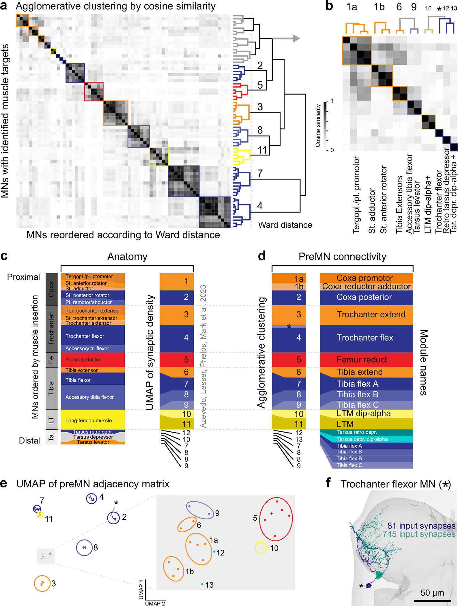
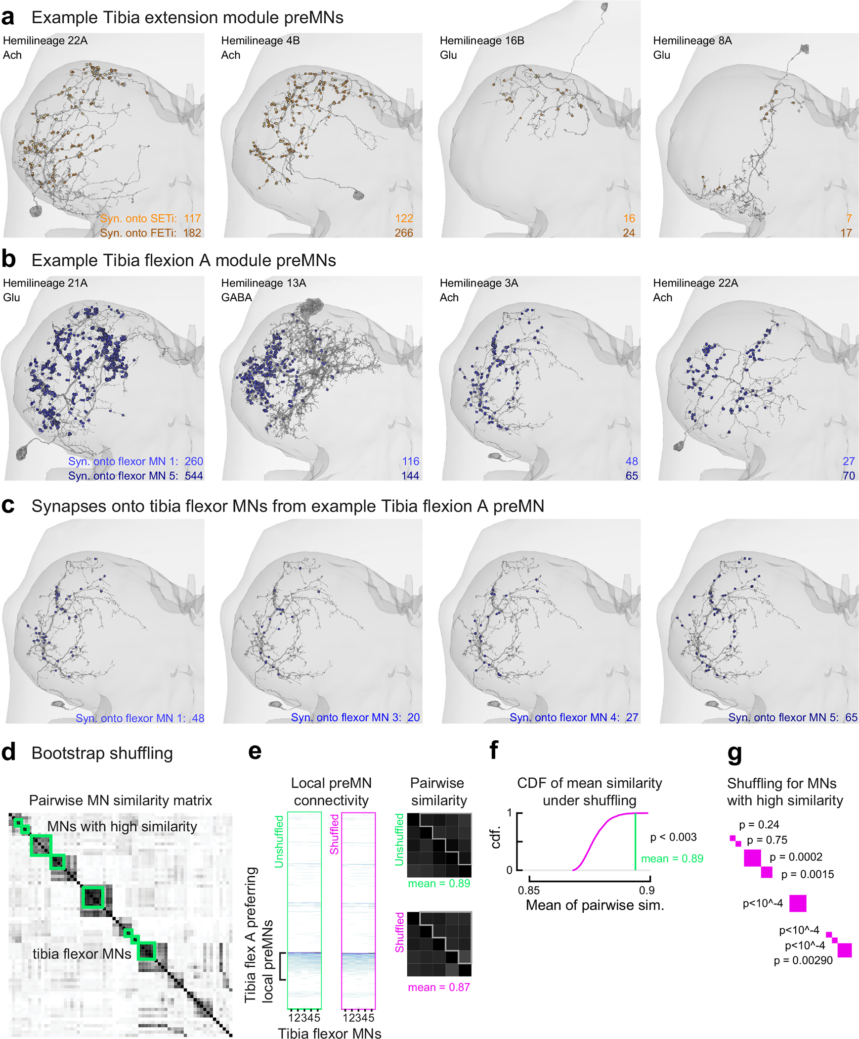
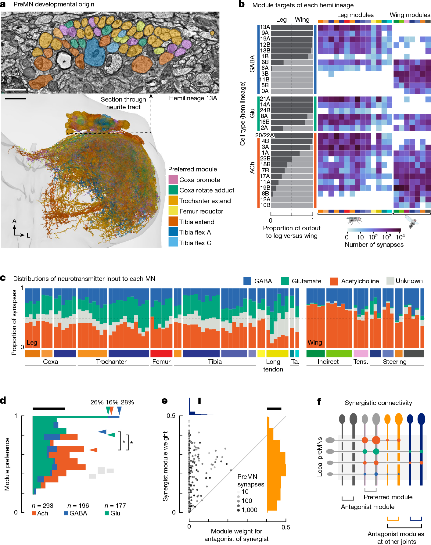
Animal movement is controlled by motor neurons (MNs), which project out of the central nervous system to activate muscles¹. MN activity is coordinated by complex premotor networks that facilitate the contribution of individual muscles to many different behaviours^2-6. Here we use connectomics⁷ to analyse the wiring logic of premotor circuits controlling the Drosophila leg and wing. We find that both premotor networks cluster into modules that link MNs innervating muscles with related functions. Within most leg motor modules, the synaptic weights of each premotor neuron are proportional to the size of their target MNs, establishing a circuit basis for hierarchical MN recruitment. By contrast, wing premotor networks lack proportional synaptic connectivity, which may enable more flexible recruitment of wing steering muscles. Through comparison of the architecture of distinct motor control systems within the same animal, we identify common principles of premotor network organization and specializations that reflect the unique biomechanical constraints and evolutionary origins of leg and wing motor control.

Extended Data Fig. 1 |. Detailed properties of individual leg and wing MNs.

a, Number of input synapses on each leg MN. MNs are ordered by the muscle they innervate, from proximal coxa muscles in the thorax to distal tarsus muscles located in the tibia. b, Number of input synapses on each wing MN. Indirect MNs are shown first, direct MNs are ordered according to sclerite. c, Fraction of synapses on each leg MN broken down by cell class (see Methods). d, Fraction of synapses on each wing MN broken down by cell class. e, Number of preMNs presynaptic to each leg MN. f, Number of preMNs presynaptic to each wing MN. g, h, Fraction of presynaptic partners from each cell class. Presynaptic partners include proofread neurons only, so fragments are not included. On average, each MN receives 3,641 input synapses from 188 preMNs (using a 3-synapse threshold) and each preMN synapses onto 6 MNs (7.2 ± 7.4 sd. for leg preMNs, 5.1 ± 3.1 for wing preMNs). i, j, MN volume. k, MN volume vs. surface area for leg MNs (left) and wing MNs (right). Wing MNs tend to have thicker neurites, explaining the steeper relationship. The thick b1 wing steering MN is the outlier.

Extended Data Fig. 2 |. Agglomerative hierarchical clustering of leg MNs according to premotor connectivity.

a, Hierarchical clustering of MNs based on the cosine similarity of the columns of the premotor connectivity matrix (Fig. 2d). The scipy.cluster AgglomerativeClustering algorithm minimizes the sum of squared distances in each cluster (Ward, scikit-learn). The algorithm identifies seven clear clusters numbered according to the proximal-to-distal origins and insertion points of the innervated muscles (right). b, Magnification of seven additional clusters at the top left of the similarity matrix. The muscle targets of MNs in each cluster are indicated below. We remain uncertain about which of four MNs innervate the tergopleural vs. the pleural promotor muscles that insert on the anterior aspect of the coxa (cluster 1a). c, In Azevedo et al., we identified the muscle targets of each MN by comparing anatomical criteria (left). We performed UMAP clustering of the density of input synapses in 3D onto each MN, as an independent, quantitative verification of our anatomical assignments (right). This analysis revealed surprising features that are corroborated by analyzing preMN connectivity here. Specifically, accessory tibia flexor MNs split into 3 distinct clusters, clusters 7, 8, and 9, where the four accessory tibia flexors in cluster 7 clustered with the five main tibia flexor MNs. Additionally, four of the six tarsus MNs clustered with the same groups, one in cluster 7, two in cluster 8, and 1 in cluster 9 (see numbers at bottom). A fifth tarsus MN, the retro depressor MN, clustered on its own (cluster 12). The final tarsus MN clustered with the small LTM MNs in cluster 10; all three are known to express dip-alpha (Venkatasubramanian et al.). d, Clusters based on premotor connectivity from a and b. The differences from the UMAP of synapse density include: promotor MNs of the coxa (cluster 1a) clustered separately from the adductor and rotator MNs (cluster 1b); the tarsus depressor MN (cluster 13) clustered separately from the two dip-alpha-positive LTM MNs (cluster 10); a small MN clustered in a separate cluster labeled with an asterisk (*), depicted in f. Names for each module are given on the right. e, UMAP embedding of the columns of the premotor connectivity matrix (Fig. 2d). This clustering does not rely on cosine similarity and largely corroborates the agglomerative clustering. f, Two trochanter flexor MNs with somas on the posterior cortex of the neuropil. In total, six MNs have somas on the dorsal cortex. Four of these neurons innervate the sternal posterior rotator muscle. We argued in Azevedo et al. that the remaining two MNs innervate the trochanter flexor muscle because we observed two axons enter the proximal fibers of the muscle in the X-ray data. The larger of the two MNs (green) clustered with the trochanter flexor MNs according to both the hierarchical clustering and the UMAP embedding. The MN indicated by the asterisk (blue) receives approximately 10X fewer synapses, perhaps explaining why it either clustered by itself (b) or with the sternal rotator MNs (e). In summary, in the paper, we include the (*) MN with the Trochanter flex MNs.

Extended Data Fig. 3 |. Similarity of wing MNs creates separable modules through agglomerative clustering.

a, Cosine similarity matrix for all wing MNs. Axes are symmetric, each row/column is an MN. (Right) The agglomerative clustering dendrogram along with the threshold at which clusters are separable. Colored branches on the dendrogram depict different modules, not muscles. b, Similarity scores for each pair of wing MNs. Indirect MNs are separated from direct and tension MNs to better show the distribution of similarity scores of direct and tension MNs. c, Schematic showing how ordering by anatomy (left) relates to agglomerative clustering by cosine similarity (right). d, UMAP does not separate the wing MNs by connectivity, possibly because their synaptic input weights are not stereotyped (or proportional) from preMNs. Data points are colored post-hoc according to the agglomerative clustering results.

Extended Data Fig. 4 |. Local PreMNs drive MN cosine similarity and modularity, for wing and leg systems.

a, Cumulative density functions (CDFs) of module preference for individual preMNs targeting leg MNs, separated by preMN cell class. Gray indicates ten overlaid example CDFs randomly selected from shuffling the columns of each row of the connectivity matrix. Right, Total MN synapses (y-axis) vs. module preference of local preMNs. Pearson’s r for each cell class is shown, p < 10⁻¹³. PreMNs with fewer MN synapses have a slight tendency to contact a single module. b, Fraction of MN input synapses (each bar) from local preMNs that prefer that MN’s module (gray) vs. prefer a different module (white). PreMN synapses onto a preferred module account for 62.2% of synapses onto leg MNs. c, Cosine similarity matrices for leg MNs, calculated using synapses from preMNs of each cell class. Modules found in Extended Data Fig. 2 are shown at left and right. Below each matrix is a color bar indicating clusters found by performing the same agglomerative clustering algorithm on the matrix above. Only local preMN connectivity gives the same clusters as using all preMNs. d, CDFs of pairwise similarity of MNs within modules defined in Extended Data Fig. 2 (dark lines) vs. across modules (light colors). Right, the area under the curve (AUC) measures the overlap of the CDFs, with 0.5 indicating similar CDFs, and 1 indicating complete separation (see Methods). Gray bars show the improvement in the AUC if the clusters shown below the similarity matrices in c are used instead. Together, these analyses show that local neurons are responsible for the modularity of MNs. Other classes of preMNs tend to prefer a single module (a) but can make select synapses across modules. e, Module preference for individual preMNs targeting wing MNs, as in a. f, Fraction of input synapses on wing MNs from local preMNs that preferentially target each MN’s module (gray) vs a different module (white). PreMN synapses onto a preferred module account for 75.7% of synapses onto wing MNs. g, Cosine similarity matrices for indirect (power) MNs, calculated using synapses from preMNs of each cell class. Indirect muscles are divided into two antagonistic modules: dorsal longitudinal muscles (DLMs, dark green) and dorso-ventral muscles (DVMs, light green). They share common input from all cell classes except sensory axons, from which they receive few synapses. h, Pairwise similarity of indirect MNs within modules, based on connectivity of each cell class. i, Similarity matrices for tension and direct (steering) MNs. j, Pairwise similarity of indirect MNs within (dark line) vs. across (light) modules, for each preMN cell class. Colors are indicated in e.

Extended Data Fig. 5 |. Example leg preMNs, their synapses onto motor modules, and impact of proportional connectivity on MN similarity.

a, The location of synapses (spheres) from example preMNs that preferentially synapse onto the SETi (light orange) and FETi (dark orange) tibia extensor MNs. Each preMN has a different morphology and makes more synapses onto FETi than onto SETi. b, Example preMNs that preferentially synapse onto the five tibia flexor MNs in the Tibia flex A module (different shades of blue spheres). c, A single example preMN from b, showing the locations of synapses onto four of the five tibia flexor MNs in the module. The preMN makes more synapses onto the largest neuron, with extra synapses distributed throughout the processes. d, Bootstrap shuffling of module connectivity (see Methods for details). This analysis is similar to Fig. 4h, but for only the largest neurons with the highest similarity (green squares), where high MN similarity reflects proportional preMN weights onto each MN in the module, as in a-c. e, Left, the unshuffled synapse counts from all local preMNs onto the Tibia Flex A MNs; middle, the same matrix with example shuffled synapse counts from the module-targeting preMNs; right, the resulting MN similarity matrices, highlighting the pairwise similarities in the upper triangle. f, The cumulative probability density function (cdf) of the mean pairwise MN similarity for N = 10,000 shuffling repeats, compared to the actual mean. The actual mean is larger than 99.7% of the shuffled instances. g, The bootstrap p-value for the regions of high MN similarity. The high p-values indicate pairs of neurons with small differences in their total synaptic input, such that shuffling the proportional synapses does not disrupt a large difference like exists for the FETi and SETi in a.

Extended Data Fig. 6 |. Leg modules that include biarticular muscles have more variable module connectivity.

a, Principal Components Analysis of the connections between local preMNs and their preferred motor module. Dots and dark gray bars indicate the percent of the module connectivity variance that is explained by a single principal component, for each leg and wing module. The first principal component was sufficient to explain the majority (>80%) of the variance within most leg motor modules. The percentages of variance explained within modules for the wing power MNs were also high (>90%). For both leg modules and the modules of the wing power muscles, the only significant dimension of variation (captured by the first component alone) was simply the overall preMN output onto the modules. By contrast, the first principal component explained only 63%, 55%, 70%, 87%, and 67% of the variance for the tension, steering A, steering B, C and D modules, respectively. This analysis supports our observation that wing module connectivity is not proportional, from Fig. 4h. Here, we further dissect the PCA analysis to show that leg modules that are composed of motor units with more biomechanical diversity have more variable connectivity, in support of our conclusions about the differences between leg and wing connectivity. b, The first principal component for the Trochanter extend module explains less of the variance than for most other leg modules. If the module is separated according to muscle target, the first PC explains more of the variance in the connectivity onto MNs targeting each muscle. c, MNs innervating the sternotrochanter, tergotrochanter, and trochanter extensor muscles. d, Individual traced muscle fibers from the X-ray tomography image volume. The Trochanter extend module contains the biarticular tergotrochanter muscle, which originates at the dorsal thoracic cuticle, crosses the body-coxa joint and extends the trochanter; and the biarticular sternotrochanter muscle, which originates on the ventral thoracic cuticle, crosses the body-coxa joint and extends the trochanter (Azevedo et al.). Note, we adopted the muscle nomenclature from the literature (Miller, 1950). All three muscles insert on the same tendon, so an alternative naming scheme would call these three parts of the same muscle, like the three parts of the human triceps brachii muscle. e, When MNs innervating the biarticular long tendon muscle (LTM) are separated by anatomy, the first PC explains more of the connectivity onto MNs targeting each muscle. f, Four groups of LTM neurons. The DIP-α LTM MNs are small, lack a medial projection, express DIP-α, and one targets the femur LTM while the other targets the tibia (Venkatasubramanian et al.). The specific muscle targets of two other smaller LTM MNs are unknown. g, Traced muscle fibers of the LTM. The LTM is composed of two muscles, one in the femur and one in the tibia, that both insert on the long tendon that crosses multiple articulations to insert on the claw at the tip of the tarsus (Radnikow and Bässler, 1991). h, Subdivision of coxa modules, for comparison with biarticular modules. Posterior modules (blue), Anterior modules (orange). Breaking the posterior module into MNs innervating the remotor/abductor muscle or the posterior rotator muscles increases the projection onto the first PC. Excluding a single MN from the coxa promotion module (orange) increases the projection onto the first PC. i, MNs innervating the coxa muscles in the thorax. Black arrowhead indicates the primary neurite of the excluded coxa promotor MN. j, Coxa muscles in the thorax. We are uncertain about how many MNs innervate the tergopleural vs. the pleural promotor muscles, as the axons are not visible in the X-ray tomography images. The excluded promotor MN receives 4,056 total synapses (compared to 1,484, 4,056, and 6,450 for the other promotor MNs) and has high cosine similarity with the rotator and adductor MNs (Extended Data Fig. 4c). This analysis suggests that the excluded preMN receives input from slightly different sources than the other preMNs. We speculate that perhaps the excluded promotor MN exits the DProN nerve and innervates the pleural promotor, while the others innervate the tergopleural promotor. In short, the leg modules with more variable input, as measured by PCA, include motor units with more complex biomechanics.

Extended Data Fig. 7 |. Example neurons from each premotor hemilineage.

Example preMNs from each premotor hemilineage. See Supplemental Table 3 for links to view entire premotor populations of each hemilineage in Neuroglancer, an online tool for viewing connectomics datasets.

Fig. 1 |. Reconstruction of synaptic inputs to identified leg and wing MNs in Drosophila.

a, Automated neuron segmentation and synapse prediction in a serial-section electron microscopy (EM) volume of an adult female VNC. The VNC contains the cell bodies and dendrites of MNs controlling the leg (left, n = 69) and wing (right, n = 29). Axons extend from the VNC to innervate muscles. Example electron microscopy image shows automated synapse predictions, with presynaptic sites labelled by yellow dots and postsynaptic sites by red dots. Scale bars, 100 μm (middle), 1 μm (right). b, Identification of muscle targets of each leg MN. Briefly, reconstructed electron microscopy neurons (top left) were compared using X-ray tomography of the leg (right) and light-microscopy images of genetically identified MNs in both the VNC (bottom left) and leg (middle; green fluorescent protein and cuticle autofluorescence in green, phalloidin in magenta). A clone of a trochanter flexor MN labelled by VT063626-Gal4 (ref. 18) with axon expression in the trochanter flexor muscle in the coxa; the axon travels in the ventral prothoracic nerve. White arrowhead indicates a sensory axon in the prothoracic leg nerve, illustrating that not all Gal4 lines are specific for MNs. Scale bar, 50 μm. c, Schematic of the 18 muscles controlling the front leg. d, Flight musculature, separated according to muscle physiology and/or insertion anatomy. e, Reconstructed MNs that extend and flex the tibia. Scale bar, 100 μm. f, Reconstructed wing MNs. Scale bar, 100 μm. g, Input synapses versus surface area for leg MNs (synapse density, 0.45 synapses μm⁻², r = 0.94, P < 10⁻³³). h, Input synapses versus surface area for direct and tension wing MNs (density, 0.41 synapses μm⁻², r = 0.90, P < 0.10⁻³, excluding the outlier b1 MN; Methods). i, Input synapses versus surface area for indirect wing MNs (density, 0.24 ± 0.02 synapses μm⁻², r = 0.98, P < 10⁻⁷). acc., accessory; PS, pleurosternal; tib., tibia; TP, tergopleural; VProN, ventral prothoracic nerve; FETi, fast tibia extensor; SETi, slow tibia extensor.

Fig. 2 |. The majority of synaptic input to MNs is derived from local interneurons.

a, Schematized premotor connectivity matrix. PreMNs (rows) are coloured according to cell class; MNs (columns) are grouped by their distinct muscle targets (shades of orange and blue). b, Examples of descending (desc.), ascending (asc.), intersegmental (interseg.) and local leg preMNs; intersegmental leg preMNs receive input from other neuromeres. Scale bar, 100 μm. c, Example intersegmental and local wing preMNs; intersegmental wing preMNs receive input from leg neuromeres. d, Premotor connectivity matrix for the left T1 leg. The colour of each element indicates log₁₀(n + 1) of the number of synapses from each preMN (row) onto each MN (column). Note that the log scale makes differences appear smaller than they are. Grey vertical lines delineate muscle targets, from proximal to distal, indicated by colour (top). PreMNs are ordered (1) by cell class, (2) by MN targets and (3) by total synapses onto all MNs. The connectivity matrix shows only synapses from fully proofread neurons; 19,349 synapses from fragments account for 8.3% of the left front leg premotor connectome (Methods). e, Same as d, for wing MNs; 11,966 synapses from fragments account for 7.6% of the left wing premotor connectome. f, Fraction of total synaptic input from each cell class onto leg or wing MNs. Fragments do not belong to any class, because they have not been attached to a primary neurite via proofreading. Fe, femur; LT, long-tendon muscle.

Fig. 3 |. PreMNs target specific groups of MNs, forming motor modules.

a, Illustration of how preMN input patterns determine cosine similarity. b,c, Similarity is the dot product of the normalized column vectors (MNs) in premotor space (black arrows) on the unit sphere (grey). b, Similar normalized synaptic weights from the same preMNs yield a similarity near 1. c, Different weights from the same preMNs yield lower similarity. d, Pairwise similarity matrix. Agglomerative clustering defines groups of similar MNs (that is, motor modules). e, Leg MN similarity matrix. Rows, muscle innervation of each MN; columns: motor modules. Labels A, B and C indicate three separate modules of tibia flexor and accessory tibia flexor MNs (Extended Data Fig. 2). Pl., pleural; St., sternal; Ter., tergo; Tergopl., tergopleural; Tr., trochanter; Ta., tarsus. f, Wing MN similarity matrix. Inset shows direct MNs reordered by module structure. tpn, third tergopleural motor neuron^,. g, Steering modules contain muscles that attach to distinct sclerites. h, Module preference for cell classes that account for about 80% of premotor input. Vertical arrowheads indicate the fraction of preMNs that synapse onto a single module; horizontal arrowheads indicate median module preference. Grey box represents the range of median module preference when rows of the connectivity matrix are shuffled (n = 10⁴ shuffles). Grey dots represent total number of MN synapses (log scale) for individual preMNs. Module preference is not strongly correlated with total MN synapses (leg preMNs: Pearson’s r = −0.29, P < 10⁻³⁰; wing preMNs: r = −0.18, P < 10⁻¹⁴). i, Similarity of MNs within modules for all preMNs, or a single class. Left, within-module leg MN similarity is lower when considering only intersegmental or descending preMNs (P < 10⁻²⁴, Kruskal–Wallis non-parametric one-way analysis of variance (ANOVA); Conover’s post hoc pairwise test with Holm correction for multiple comparisons: *P < 10⁻⁶). Right, within-module similarity of wing steering MNs (excluding indirect and tension muscle MNs) is generally lower than for leg MNs.

Fig. 4 |. Local preMN connectivity differs between leg and wing steering motor modules.

a, Illustration of proportional connectivity. PreMN output is the sum of a preMN synapses onto the module. b, Synaptic weights from module-preferring local preMNs onto the slow (SETi) and fast (FETi) tibia extensor MNs are proportional to MN size. c, Same as b, for the tibia flex A module. Tibia flex A MNs are ordered by surface area. Bold indicates MNs previously characterized using electrophysiology. The fraction of preMN output onto the largest MN is significantly larger than that onto smaller MNs (P < 10⁻⁴, Kruskal–Wallis non-parametric one-way ANOVA; Conover’s post hoc pairwise test with Holm correction for multiple comparisons: ***P < 10⁻²⁸, *P = 0.012). d, Wing steering motor module connectivity is not proportional to MN size. e, Same as b, for wing steering modules A and B. f, Illustration of the connectivity motif for steering module C. g, Same as b, for steering module C. h, Average cosine similarity (black dots) compared with average cosine similarity when synapse weights from local preMNs onto their preferred module are shuffled (grey probability density function (PDF), n = 10,000 shuffles). The measured mean is higher than 99% of PDF in all cases except for coxa promotors (left, larger than 98.3%), steering module B (62%) and steering modules A and D (higher than 2 and 5% of shuffles, respectively). i, The tibia flex A module produces torque on the tibia. Measurements of tibia force produced by single spikes in the 2 and 5 MNs in c. j, Schematic of muscles innervated by steering module B. Different origins and attachments suggest that cocontraction of muscles can have variable biomechanical effects.

Fig. 5 |. PreMNs from diverse developmental lineages synapse on MNs in each motor module.

a, PreMNs from an example hemilineage (13A, GABAergic), coloured according to their preferred leg motor module. Scale bars, 1 μm (top), 20 μm (bottom). b, Left, proportion of total synapses from all local and intersegmental preMNs in each hemilineage onto leg MNs versus wing MNs. Right, total synapses onto MNs in each leg or wing module. c, Proportion of synaptic input to MNs from cholinergic (green), glutamatergic (yellow), GABAergic (pink) and unidentified (light grey) hemilineages. Only local and intersegmental preMNs are included in this analysis (Methods). Tens., tension. d, Module preference of local preMNs, by hemilineage neurotransmitter. Horizontal arrowheads indicate the median module preference (P = 0.0013, Kruskal–Wallis non-parametric one-way ANOVA; Conover’s post hoc pairwise test with Holm correction for multiple comparisons: *P = 0.002). Grey rectangles indicate the range of medians when preMN connections are shuffled. Vertical arrowheads denote the percentage of neurons that target a single module. Scale bar, 20 preMNs. e, Module weights for synergist module (y axis, orange histogram) versus the antagonist of the synergist module (x axis, blue histogram; Methods). Dot hue indicates total synapses onto all MNs. Scale bars, 100 preMNs (vertical), 50 preMNs (horizontal). f, Schematic of preMN targeting synergist module while avoiding antagonist modules.

References

1. Kernell D The Motoneurone and Its Muscle Fibres (Oxford Univ. Press, 2006).
1. Marshall NJ et al. Flexible neural control of motor units. Nat. Neurosci. 25, 1492–1504 (2022). - PMC - PubMed
1. Henneman E, Clamann HP, Gillies JD & Skinner RD Rank order of motoneurons within a pool: law of combination. J. Neurophysiol. 37, 1338–1349 (1974). - PubMed
1. Tresch MC, Saltiel P, d’Avella A & Bizzi E Coordination and localization in spinal motor systems. Brain Res. Rev. 40, 66–79 (2002). - PubMed
1. Ting LH & Macpherson JM A limited set of muscle synergies for force control during a postural task. J. Neurophysiol. 93, 609–613 (2005). - PubMed
MeSH terms
LinkOut - more resources