A Compact, Low-Cost, and Low-Power Turbidity Sensor for Continuous In Situ Stormwater Monitoring

Abstract

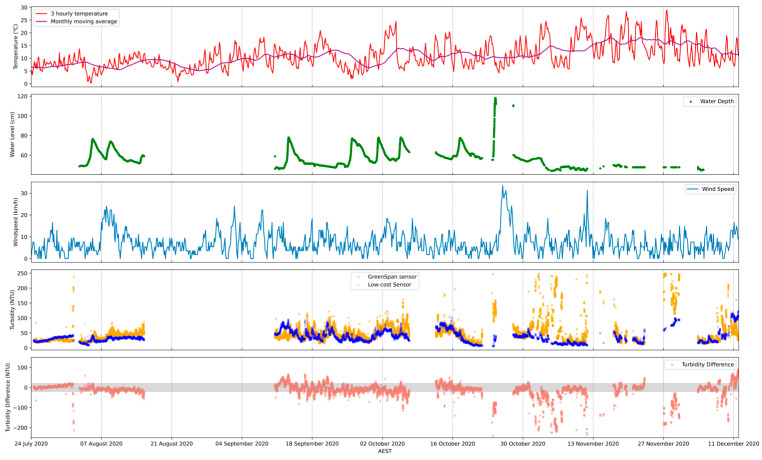
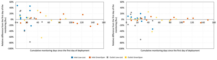
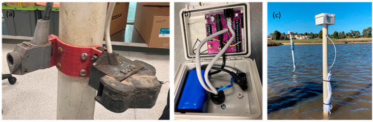
Turbidity stands as a crucial indicator for assessing water quality, and while turbidity sensors exist, their high cost prohibits their extensive use. In this paper, we introduce an innovative turbidity sensor, and it is the first low-cost turbidity sensor that is designed specifically for long-term stormwater in-field monitoring. Its low cost (USD 23.50) enables the implementation of high spatial resolution monitoring schemes. The sensor design is available under open hardware and open-source licences, and the 3D-printed sensor housing is free to modify based on different monitoring purposes and ambient conditions. The sensor was tested both in the laboratory and in the field. By testing the sensor in the lab with standard turbidity solutions, the proposed low-cost turbidity sensor demonstrated a strong linear correlation between a low-cost sensor and a commercial hand-held turbidimeter. In the field, the low-cost sensor measurements were statistically significantly correlated to a standard high-cost commercial turbidity sensor. Biofouling and drifting issues were also analysed after the sensors were deployed in the field for more than 6 months, showing that both biofouling and drift occur during monitoring. Nonetheless, in terms of maintenance requirements, the low-cost sensor exhibited similar needs compared to the GreenSpan sensor.

Keywords: IoT; real-time; sediment; stormwater management; turbidity; urban water.

Figure A1

Regression of measured turbidity and low-cost sensor reading results. The blue dots indicate the measuring results vs the actual turbidity reading, the redline is the trend line of the best fits of the results, and the red words displayed in the graphs indicate the equation of the trendline and the R square value.

Figure A2

Turbidity and weather time series data at wetland inlet. From the top to the bottom: 1. Temperature during the monitoring period, with the red line indicating the 3 hourly temperature and the purple line representing the monthly temperature moving average; 2. Water level at the monitoring point; 3. Hourly wind speed; 4. Turbidity sensor data from both sensors and the rainfall data; and 5. Turbidity difference (low-cost sensor readings minus Greenspan sensor readings) between both sensors. The positive values show greater low-cost sensor data and the negative values show greater Greenspan sensor data; the shaded area shows ±20 NTU difference, which is 97% of the total data.

Figure A3

Turbidity and weather time series data at wetland outlet. From the top to the bottom: 1. Temperature during the monitoring period, with red line indicating the 3 hourly temperature and purple line representing the monthly temperature moving average; 2. Water level at the monitoring point; 3. Hourly wind speed; 4. Turbidity sensor data from both sensors and the rainfall data; and 5. Turbidity difference (low-cost sensor readings minus Greenspan sensor readings) between both sensors. The positive values show greater low-cost sensor data and negative values show greater Greenspan sensor data; the shaded area shows ±20 NTU difference which 73.3% of the total data.

Figure A4

Debris and aquatic animal (river snails) in the sensor cover and on the sensor surface.

Figure A5

Relative difference between the after-cleaning turbidity and the before-cleaning turbidity for each sensor; 25th percentile turbidity level (left) and 75th percentile turbidity level (right).

Figure A6

Relative difference between the after-cleaning turbidity and the after-cleaning turbidity for each sensor; 25th percentile turbidity level (left) and 75th percentile turbidity level (right).

Figure 1

(a) circuit diagram of the innovative turbidity sensor; (b) PCB 3D view with dimension of the turbidity sensor (left for front side, right for back side); (c) 3D printed LED and phototransistor holder to arrange them at fixed positions, and each component has a 45 degree angle holder that makes the LED and phototransistor face each other with a 90 degree angle; (d) the top view of the PCB arrangement in the sensor housing, with the LED and phototransistor holder fixed in front of the housing and the PCB sitting in the middle of the sensor case; and (e) assembled turbidity sensor with a proper 3D printed housing, without cover assembled (top) and with cover assembled (bottom).

Figure 2

(a) low-cost sensors fixed on the PVC pipe; (b) low-cost sensor logger box; and (c) low-cost sensor package in the wetland.

Figure 3

Regression of measured turbidity and the low-cost sensor’s outputs. The blue dots indicate the measuring results vs. the actual turbidity reading, the red dash line is the trend line of the best fits of the results, and the red words displayed in the graphs indicate the equation of the trendline and the R square value.

Figure 4

Time series data (after cleaning) and result difference between low-cost sensor and GreenSpan sensor. From the top to the bottom: the first and third subplots show the time series plot of the inlet data and outlet data, respectively; the second and the forth subplots show the turbidity difference (low-cost sensor readings minus Greenspan sensor readings) between both sensors for inlet and outlet, respectively; the positive values show greater low-cost sensor data and negative values show greater Greenspan sensor data; and the shaded area shows ±20 NTU difference, which is 97% of the total data at inlet and 73% at the outlet.

Figure 5

Plot of the GreenSpan sensor results vs the low-cost sensor results at both wetland inlet (left) and outlet (right). The black dash line shows the identity line, and the red dash line is the best fit line for the data series. The linear trendline equation is shown in red colour; for the inlet trendline, the estimated slope is 0.75 [95% CI: 0.73, 0.76], the estimated intercept is 2.24 [95% CI: 1.92, 2.57], and for the outlet trendline, the estimated slope is 0.22 [95% CI: 0.21, 0.23], and the estimated intercept is 2.24 [95% CI: 25.88, 26.89]. The R value and p-value of Pearson test are shown in the diagram respectively.

Figure 6

Plots of biofouling analysis and drift analysis. The left two graphs show the biofouling results, the top left graph is the boxplots of the relative difference (R_bio) of biofouling effect, and the bottom left graph shows the relative difference (R_bio) against the cumulative monitoring days in each specific monitoring period. Negative values mean the “after-cleaning” turbidity is smaller than the “before-cleaning” turbidity in a specific raw reading, and positive values mean the “after-cleaning” turbidity is greater than the “before-cleaning” turbidity in a specific raw reading. The right two graphs show the drift results, the top left graph is the boxplots of the relative difference of drift effect, and the top left graph shows the relative difference of the drift effect against the cumulative monitoring days since the sensor deployment. Negative values mean the “after-cleaning” turbidity before sensor is deployed is smaller than the “after-cleaning” turbidity after sensor is deployed in a specific raw reading, and positive values mean the “after-cleaning” turbidity before sensor is deployed is greater than the “after-cleaning” turbidity after sensor is deployed in a specific raw reading. Wilcoxon Rank Sum test results of comparing the box plots of low-cost sensor and GreenSpan sensor for both biofouling and drift effects are also shown below the box plots. Due to the axis limitation, some outliers are not shown in the boxplots (1 outlier for biofouling analysis 25 percentile, 1 outlier for drift analysis 25 percentile, and 1 outlier for drift analysis 50 percentile). The turbidity ranges for different percentile at both inlet and outlet are also presented on the top of the top graphs. For the plots of 25 percentile and 75 percentile in biofouling and drift effect against deployment period, please see Appendixes D and E.

References

1. Gaffield S.J., Goo R.L., Richards L.A., Jackson R.J. Public health effects of inadequately managed stormwater runoff. Am. J. Public Health. 2003;93:1527–1533. doi: 10.2105/AJPH.93.9.1527. - DOI - PMC - PubMed
1. Landsberg J.H. The effects of harmful algal blooms on aquatic organisms. Rev. Fish. Sci. 2002;10:113–390. doi: 10.1080/20026491051695. - DOI
1. Loucks D.P., Van Beek E. Water Resource Systems Planning and Management: An Introduction to Methods, Models, and Applications. Springer; Berlin/Heidelberg, Germany: 2017.
1. Withanachchi S.S., Ghambashidze G., Kunchulia I., Urushadze T., Ploeger A. Water quality in surface water: A preliminary assessment of heavy metal contamination of the Mashavera river, Georgia. Int. J. Environ. Res. Public Health. 2018;15:621. doi: 10.3390/ijerph15040621. - DOI - PMC - PubMed
1. Jaskuła J., Sojka M., Fiedler M., Wróżyński R. Analysis of spatial variability of river bottom sediment pollution with heavy metals and assessment of potential ecological hazard for the Warta river, Poland. Minerals. 2021;11:327. doi: 10.3390/min11030327. - DOI
LinkOut - more resources