Time of sample collection is critical for the replicability of microbiome analyses

Abstract

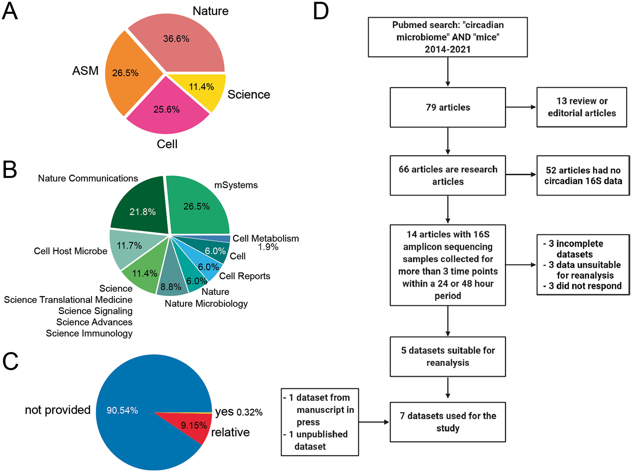
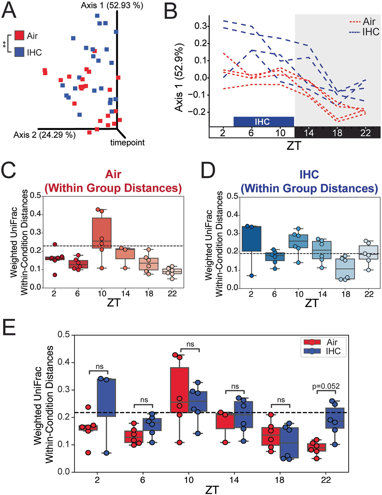
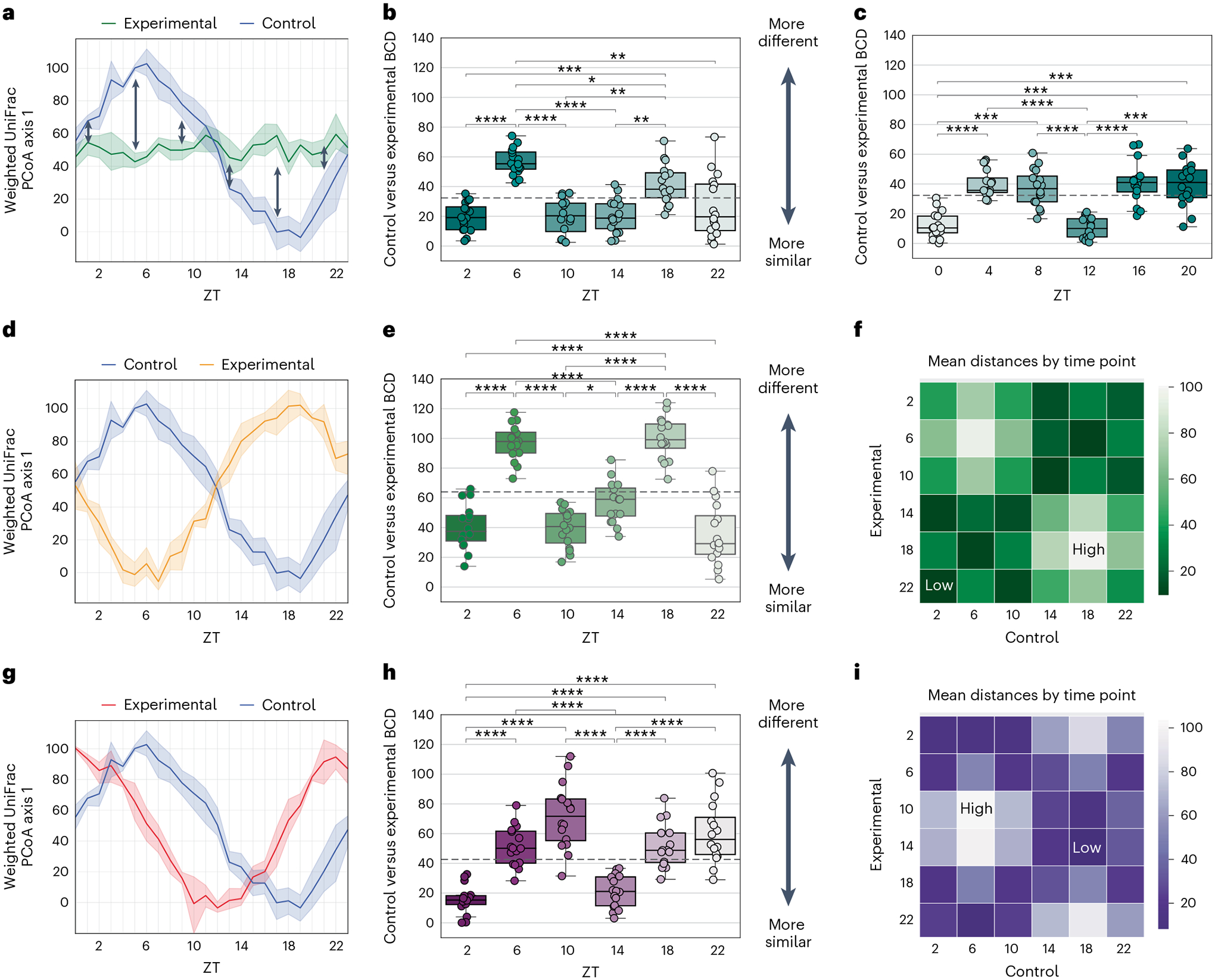
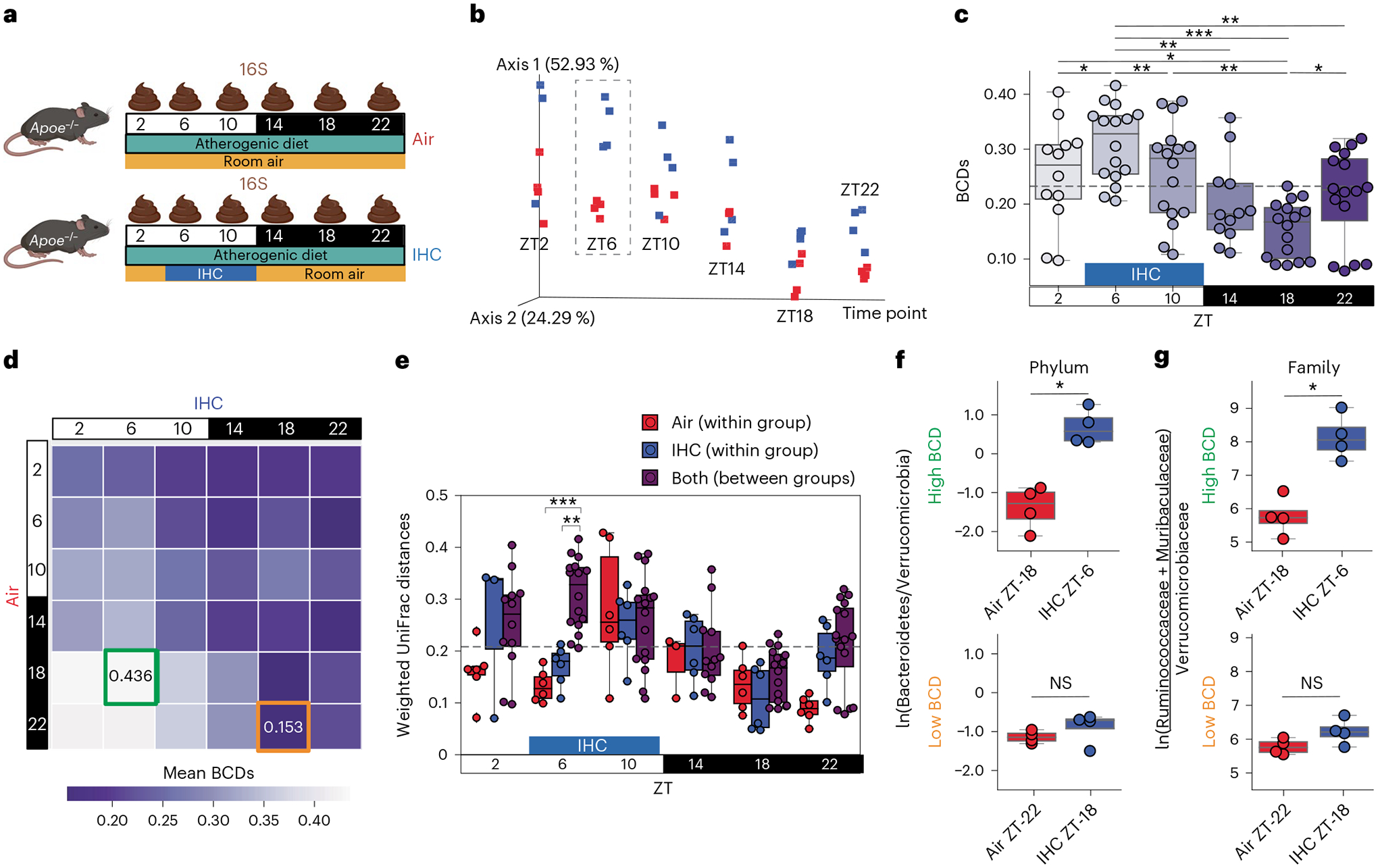
As the microbiome field moves from descriptive and associative research to mechanistic and interventional studies, being able to account for all confounding variables in the experimental design, which includes the maternal effect¹, cage effect², facility differences³, as well as laboratory and sample handling protocols⁴, is critical for interpretability of results. Despite significant procedural and bioinformatic improvements, unexplained variability and lack of replicability still occur. One underexplored factor is that the microbiome is dynamic and exhibits diurnal oscillations that can change microbiome composition^5-7. In this retrospective analysis of 16S amplicon sequencing studies in male mice, we show that sample collection time affects the conclusions drawn from microbiome studies and its effect size is larger than those of a daily experimental intervention or dietary changes. The timing of divergence of the microbiome composition between experimental and control groups is unique to each experiment. Sample collection times as short as only 4 hours apart can lead to vastly different conclusions. Lack of consistency in the time of sample collection may explain poor cross-study replicability in microbiome research. The impact of diurnal rhythms on the outcomes and study design of other fields is unknown but likely significant.

Extended Data Fig. 1 |. Microbiome Literature Review.

A) 2019 Literature Review Summary. Of the 586 articles containing microbiome (16 S or metagenomic) data, found as described in the methods section, the percentage of microbiome articles from each of the publication groups. B) The percentage of microbiome articles belonging to each individual journal in 2019. Because the numerous individual journals from Science represented low percentages individually, they were grouped together. C) The percentage articles where collection time was explicitly stated (yes: 8 AM, ZT4, etc.), implicitly stated (relative: ‘before surgery’, ‘in the morning’, etc.), or unstated (not provided: ‘daily’, ‘once a week’, etc.). D) Meta-Analysis Inclusion Criteria Flow Chart. Literature review resulting in the five previously published datasets for meta-an alysis^,,–.

Extended Data Fig. 2 |. Single Time Point (Non-Circadian) Example.

A) Weighted UniFrac PCoA Plot - modified example from Moving Pictures Qiime2 tutorial data [https://docs.qiime2.org/2022.11/tutorials/moving-pictures/]. Each point is a sample. Points were coloured by body site of origin. There are 8 gut, 8 left palm, 9 right palm, and 9 tongue samples. B) Within-Condition Distances (WCD) boxplot/stripplot for each body site (n = 8–9 mouse per group per time point). C) Between Condition Distances (BCD) boxplot/stripplot for each unique body site comparison (n = 8–9 mouse per group per time point). D) All pairwise grouping comparisons, both WCD and BCD, are shown in the boxplots/stripplots (n = 8–9 mouse per group per time point). Only WCD to BCD statistical differences are shown. Boxplot centre line indicates median, edges of boxes are quartiles, error bars are min and max values. Significance was determined using a paired Mann-Whitney-Wilcoxon test two-sided with Bonferroni correction. Notation: ns (not significant) = p > 0.05, * = p < 0.05; ** = p < 0.01; *** = p < 0.001, **** = p < 0.00001.

Extended Data Fig. 3 |. Additional Analysis of Apoe−/− Mice Exposed to IHC Conditions.

A) Weighted UniFrac PCoA stacked view (same as Fig. 2b but different orientation). Good for assessing overall similarity not broken down by time point. Significance determined by PERMANOVA (p = 0.005). B) Weighted UniFrac PCoA of only axis 1 over time. C) Boxplot/scatterplot of within-group weighted UniFrac distance values for the control group (Air, n = 3–4 samples per time point). Unique non-zero values in the matrix were kept. Dotted line indicates the mean of all values presented. No significant differences (p > 0.05) found. D) Boxplot/scatterplot of within-group weighted UniFrac distance values for the experimental group (IHC, n = 3–4 samples per time point)). Unique non-zero values in the matrix were kept. Dotted line indicates the mean of all values presented. No significant differences (p > 0.05) found. E) Boxplot/scatterplot of within-group weighted UniFrac distance values for both control (Air) and experimental (IHC) groups [n = 3–4 samples per group per time point]. Mann-Whitney-Wilcoxon test with Bonferroni correction used to determine significant differences between groups. Boxplot centre line indicates median, edges of boxes are quartiles, error bars are min and max values. Notation: ns = not significant, p > 0.05; * = p < 0.05; ** = p < 0.01; *** = p < 0.001.

Extended Data Fig. 4 |. Irregular differences in diurnal rhythm patterns leads to generally minor shifts in BCD when comparing LD vs DD mice.

A) Experimental design. Balb/c mice were fed NCD ad libitum under 0:24 L:D (24 hr darkness, DD) experimental conditions and compared to 12:12 L:D (LD) control conditions. After 2 weeks, mice from each group were euthanized every 4 hours for 24 hours (N = 4–5 mice/condition) and samples were collected from the proximal small intestine (‘jejunum’) and distal small intestine (‘ileum’) contents. B) BCD for luminal contents of proximal small intestine samples comparing LD to DD mice (N = 4–5 mice/condition). Dotted line is the average of all shown weighted UniFrac distances. Significance was determined using a paired Mann-Whitney-Wilcoxon test two-sided with Bonferroni correction; notation: **** = p < 0.00001. C) BCD for luminal contents of distal small intestine samples comparing LD to DD mice (N = 4–5 mice/condition). Dotted line is the average of all shown weighted UniFrac distances. Boxplot centre line indicates median, edges of boxes are quartiles, error bars are min and max values.

Extended Data Fig. 5 |. Localized changes in BCD between luminal and mucosal contents.

A) Experimental design and sample collection for a local site study. Small intestinal samples were collected every 4 hours for 24 hours (N = 4–5 mice/condition, skipping ZT8). Mice were fed ad libitum on the same diet (NCD) for 4 weeks before samples were taken. B) BCD for luminal vs mucosal conditions (N = 4–5 mice/condition). The dotted line is the average of all shown weighted UniFrac distances. Significance is determined using the Mann-Whitney-Wilcoxon test two-sided with Bonferroni correction. C) Heatmap of mean BCD distances comparing luminal and mucosal by time point (N = 4–5 mice/condition). Highest value highlighted in navy, lowest value highlighted in gold. Boxplot centre line indicates median, edges of boxes are quartiles, error bars are min and max values. Significance was determined using a paired Mann-Whitney-Wilcoxon test two-sided with Bonferroni correction. Notation: * = p < 0.05; ** = p < 0.01; *** = p < 0.001, **** = p < 0.00001. D) Experimentally relevant log ratio, highlighting the changes seen at ZT20 (N = 4–5 mice/condition). Boxplot center line indicates median, edges of boxes are quartiles, error bars are min and max values. Significance was determined using a paired Mann-Whitney-Wilcoxon test two-sided with Bonferroni correction. Notation: * = p < 0.05; ** = p < 0.01; *** = p < 0.001, **** = p < 0.00001.

Fig. 1 |. Mock circadian data to explain and exemplify new metric BCD.

Example 1: diurnal oscillations compared to non-oscillatory. a, PCoA axis 1 over the course of a day (ZT0 at lights on). Arrows indicate what BCD is measuring. Blue indicates the control group, green indicates the experimental group. Shaded regions indicate 95% confidence interval. b, Box-plot/strip-plot of control-to-experimental BCD (n = 4 per group) at six different time points (denoted by blue-green colour). c, Box-plot/strip-plot of control-to-experimental BCD (n = 4 per group) at six alternate time points (shifted by 2 h). Example 2: opposing diurnal oscillations. d, PCoA axis 1 over the course of a day. Blue indicates control group, yellow indicates the experimental group and shaded regions indicate 95% confidence intervals. e, Box-plot/strip-plot of control-to-experimental BCD (n = 4 per group) at six different time points (denoted by green colour). f, Heatmap of mean (n = 4 per group) mock β diversity distance values by the six selected time points, calculated using only control group samples. Highest and lowest values are labelled. Example 3: offset (by 6 h/1.5 time points) diurnal oscillations. g, PCoA axis 1 over the course of a day. Blue indicates control group, red indicates experimental group and shaded regions indicate 95% confidence interval. h, Box-plot/strip-plot of control-to-experimental BCD (n = 4 per group) at six different time points (denoted by purple colour). i, Heatmap of mean (n = 4 per group) mock β diversity distance values by the six selected time points, calculated using only control group samples. Highest and lowest values are labelled. Box-plot centre line in all panels indicates median, edges of boxes represent quartiles and error bars show min and max values. Significance for all was determined using a paired, two-sided Mann–Whitney–Wilcoxon test with Bonferroni correction. *P < 0.05; **P < 0.01; ***P < 0.001; ****P < 0.00001.

Fig. 2 |. Microbiome analysis of Apoe^−/− mice exposed to IHC conditions show different outcomes depending on time point of sample collection.

a, Experimental design. n = 4 mice per group per time point; ZT2 one IHC sample rarefied out, ZT14 one air sample rarefied out. Image was created with BioRender.com. b, Weighted UniFrac PCoA lateral view, with time points as one axis. c, BCD, a subset of weighted UniFrac β-diversity distances (n = 4 mice per group per time point). Significance was determined using paired Wilcoxon rank-sum test. The BCD values in this experiment were oscillating in a circadian fashion (MetaCycle, JTK method, P < 0.001). d, BCD heatmap by time point. Replicates were collapsed by taking the mean. Highest are highlighted in green and lowest are highlighted in orange. e, Box-plot/scatter-plot of weighted UniFrac distance values for WCD for control (air, red), WCDs for experimental (IHC, blue) and BCDs (both, purple) groups (n = 4 mice per group per time point). Mann–Whitney–Wilcoxon test with Bonferroni correction used to determine significant differences between the three groups. f,g, At the peak and trough time points identified in d, the logarithmic ratios of differentially abundant key phyla of interest (n = 4 mice per group per time point) (f) and the logarithmic ratios of differentially abundant key families of interest (n = 4 mice per group per time point) (g). A Mann–Whitney–Wilcoxon test with Bonferroni correction was used to determine significant differences. The box-plot centre line in all panels indicates the median, edges of boxes show quartiles and error bars represent min and max values. NS, not significant; *P < 0.05; **P < 0.01; ***P < 0.001; ****P < 0.00001.

Fig. 3 |. Gastrointestinal regions have individual time dynamics that are influenced by diet and feeding patterns.

a, Experimental design. TRF mice were restricted to eating only between ZT13–ZT21. Time point ZT13 was collected before access to the diet was given and, thus, mice were fasted at this time point. Time points were taken every 4 h for 24 h (n = 3 mice per condition per time point from separate cages; six total time points). Every point on the box-plot + swarm-plot represents the calculated β diversity distance between a control and experimental mouse. Image was created with BioRender.com. b–d, Caecum. BCD box-plot/swarm-plot for NCD ad libitum (control) versus HFD ad libitum (b), NCD ad libitum (control) versus HFD TRF (c) and HFD ad libitum versus HFD TRF (d). e–g, Ileum. BCD box-plot/swarm-plot for NCD ad libitum versus HFD ad libitum (e), NCD ad libitum versus HFD TRF (f) and HFD ad libitum versus HFD TRF (g). The dotted line is the average/mean of all shown weighted UniFrac distances. Significance was determined using Mann–Whitney–Wilcoxon test two-sided with Bonferroni correction. h, Experimental design. Mice were fed ad libitum with either NCD or high MFD. After 5 weeks, caecal and ileal samples were collected every 4 h for 24 h (n = 3 mice per condition per time point). Image was created with BioRender.com. i, BCD for both ileal and caecal samples comparing NCD versus high MFD The dotted line is the average of all shown weighted UniFrac distances. Ileal versus caecal pairwise significance was determined using Mann–Whitney–Wilcoxon test two-sided with Bonferroni correction. Box-plot centre line indicates median, edges of boxes show quartiles and error bars indicate min and max values. Significance was determined using a two-sided Mann–Whitney–Wilcoxon test with Bonferroni correction. *P < 0.05; **P < 0.01; ***P < 0.001; ****P < 0.00001.

Fig. 4 |. Longitudinal data are also susceptible to the influence of time.

a, Experimental design and sample collection for longitudinal IHC study. During the 10 weeks of exposure to either normal room air or IHC conditions, samples were collected between ZT3 and ZT5 every 3–4 days for the duration of the study (n = 12 mice per condition). Image was created with BioRender.com. b, Faecal BCD violin plot over the course of the IHC longitudinal study. Diet switch was from NCD to an atherogenic diet (AD) and occurred on day 1. Dotted line shows the mean of all data shown. While most of the other time points are significantly different from each other, the only comparison shown is between age 10.5 weeks and 19.5 weeks, which is most relevant to our discussion. Significance was determined using a paired, two-sided Wilcoxon rank-sum test. c, Experimental design and sample collection for TRF study. Mice were fed AD either ad libitum or TRF. Samples were collected every 4 h for 24 h (n = 6 mice per condition per time point) after 1 week (early; pre-phenotype) and after 20 weeks (late; post-phenotype). Image was created with BioRender.com. d, Faecal BCD box-plot/scatter-plot for ad libitum versus TRF conditions at the early (week 1) and late (week 20) time points. Dotted line is the average of all of the weighted UniFrac distances. Significance was determined using a paired, two-sided Wilcoxon rank-sum test. e,f, BCD heatmap for early samples (e) and late samples (f). Replicates were collapsed by taking the mean. The highest value is highlighted in tan and the lowest value is highlighted in yellow. Box-plot centre line indicates median, edges of boxes show quartiles and error bars indicate the min and max values. *P < 0.05; **P < 0.01; ***P < 0.001; *****P < 0.00001.

References

1. Schloss PD Identifying and overcoming threats to reproducibility, replicability, robustness, and generalizability in microbiome research. mBio 9, e00525–18 (2018). - PMC - PubMed
1. Gilbert JA et al. Current understanding of the human microbiome. Nat. Med 24, 392–400 (2018). - PMC - PubMed
1. Knight R et al. Best practices for analysing microbiomes. Nat. Rev. Microbiol 16, 410–422 (2018). - PubMed
1. Ley RE et al. Obesity alters gut microbial ecology. Proc. Natl Acad. Sci. USA 102, 11070–11075 (2005). - PMC - PubMed
1. Deloris Alexander A et al. Quantitative PCR assays for mouse enteric flora reveal strain-dependent differences in composition that are influenced by the microenvironment. Mamm. Genome 17, 1093–1104 (2006). - PubMed