A mapped dataset of surface ocean acidification indicators in large marine ecosystems of the United States

Abstract

Mapped monthly data products of surface ocean acidification indicators from 1998 to 2022 on a 0.25° by 0.25° spatial grid have been developed for eleven U.S. large marine ecosystems (LMEs). The data products were constructed using observations from the Surface Ocean CO₂ Atlas, co-located surface ocean properties, and two types of machine learning algorithms: Gaussian mixture models to organize LMEs into clusters of similar environmental variability and random forest regressions (RFRs) that were trained and applied within each cluster to spatiotemporally interpolate the observational data. The data products, called RFR-LMEs, have been averaged into regional timeseries to summarize the status of ocean acidification in U.S. coastal waters, showing a domain-wide carbon dioxide partial pressure increase of 1.4 ± 0.4 μatm yr^-1 and pH decrease of 0.0014 ± 0.0004 yr^-1. RFR-LMEs have been evaluated via comparisons to discrete shipboard data, fixed timeseries, and other mapped surface ocean carbon chemistry data products. Regionally averaged timeseries of RFR-LME indicators are provided online through the NOAA National Marine Ecosystem Status web portal.

Fig. 1

Schematic of the procedure used to construct the ocean acidification indicator data products described by this study. Steps within each section on the right (A, B, and C) are labelled in the schematic on the left.

Fig. 2

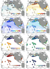
Observations used to develop ocean acidification indicator data products in the eleven U.S. large marine ecosystems (LMEs) considered in this study. LME boundaries are displayed with (a) platform-weighted fCO₂ from SOCATv2023, averaged over 1998–2022 in 0.25 degrees latitude by 0.25 degrees longitude grid cells; (b) platform-weighted fCO₂ variability from SOCATv2023, calculated as the standard deviation over time in 0.25 degrees latitude by 0.25 degrees longitude grid cells; (c) the total number months over the timeseries with at least one observation in each grid cell; (d) months of the seasonal cycle with at least one observation in each grid cell; (e) sea surface temperature from OISSTv2; (f) sea surface salinity from the CMEMS GLORYS reanalysis product; (g) wind speed from the ECMWF ERA5 reanalysis product; and (h) bathymetry from the ETOPO 2022 Global Relief Model. LME name abbreviations shown in panel (a) are provided in Table 1.

Fig. 3

Example for Gaussian Mixture Model (GMM) optimization in the North Bering Chukchi Seas (NBCS). (a) Parameters used for GMM evaluation in the NBCS, plotted against the number of GMM clusters (N). The goal of the optimization procedure was to minimize the root mean squared error, maximize the global mean silhouette score, and identify the N at which the Bayesian information criterion was no longer sharply decreasing. N = 6 was ultimately selected for the NBCS region. (b) Distribution of GMM clusters for the NBCS and (c) the probability for grid cells belonging to cluster 1 (C1).

Fig. 4

Long-term means of RFR-LME mapped OA indicators. Mapped averages of (a) pCO_2(RFR-LME), (b) C_T(RFR-LME), (c) pH_T(RFR-LME), (d) [H⁺]_T(RFR-LME), (e) Ω_ar(RFR-LME), (f) Ω_ca(RFR-LME), (g) [CO₃²⁻]_T(RFR-LME), and (h) RF_(RFR-LME) over the timeseries (1998–2022) within each LME.

Fig. 5

Seasonal means of C_T(RFR-LME). Mapped averages of C_T(RFR-LME), in the northern hemisphere (a) winter (DJF), (b) spring (MAM), (c) summer (JJA), and (d) fall (SON) over the timeseries (1998–2022) within each LME.

Fig. 6

k-fold cross-validated differences between estimated and measured fCO₂ and scaled uncertainty in fCO_2(RFR-LME), A_T(ESPER), and Ω_ar(RFR-LME). (a) Absolute differences (|ΔfCO₂|) between fCO_{2(RFR-LME-kFold)} and fCO_2(SOCAT) calculated via a k-fold cross-validation approach compared to (b) long-term average uncertainty in fCO_{2(RFR-LME-kFold)}, calculated and scaled according to the procedure in the Uncertainty estimation section. Long-term average uncertainty in (c) A_T(ESPER) and (d) Ω_ar(RFR-LME) are also shown.

Fig. 7

pCO₂ timeseries for the eleven U.S. LMEs considered in this study. Area-weighted annual (red) and monthly (black) means are presented along with envelopes of uncertainty. Uncertainties are calculated by scaling k-fold cross-validated uncertainties spatially with a two-dimensional low-pass filter, then temporally according to long-term data coverage (5-year running windows) and seasonal data coverage (3-month running windows). Average values across the timeseries are indicated by dotted lines. Note the different y-axis for each LME. For many LMEs, uncertainties are larger near the beginning of the timeseries, when SOCAT observations are less dense. Inset within each timeseries plot is a figure showing the percent of the LME represented across the seasonal cycle by grid cells that remain ice-free across the entire timeseries; these are the grid cells used to compute monthly and annual means.

Fig. 8

pH_T timeseries for the eleven U.S. LMEs considered in this study. Same as Fig. 7, except for pH_T.

Fig. 9

Ω_ar timeseries for the eleven U.S. LMEs considered in this study. Same as Fig. 7, except for Ω_ar.

Fig. 10

Comparisons between OA indicators retrieved from RFR-LME maps and those calculated from discrete observations. (a,c,e) Histograms showing differences between calculations of (a) pCO₂, (c) pH_T, and (e) Ω_ar from discrete surface (depth ≤ 10 m) observations of A_T and C_T and values of the same OA indicators from RFR-LME maps. Discrete observations that fall within the boundaries of LMEs were obtained from the GLODAPv2.2022 and CODAP-NA data products. Error statistics shown represent the median errors and the interquartile ranges of errors for each comparison. (b,d,f) Mapped differences between calculations of (b) pCO₂, (d) pH_T, and (f) Ω_ar from discrete surface (depth ≤ 10 m) observations of A_T and C_T and values of the same OA indicators from RFR-LME maps. Discrete differences are binned into 1° × 1° grid cells for this map.

Fig. 11

Summarized differences between monthly binned moored buoy pCO₂ observations and mapped pCO₂ data products. (a) Medians and (b) interquartile ranges of differences, (c) differences in seasonal amplitudes, and (d) correlations of residual values (after removing the trend and seasonal cycle) between binned moored buoy pCO₂ observations and mapped pCO₂ data products. Each of these statistics are shown as boxplots representative of all 14 mooring sites compared to each mapped product, where the boxes extend from the 25^th to 75^th percentile, the center line shows the median of the data, the whiskers extend to the most extreme data points not considered outliers, and dots denote outliers (arrows denote where outliers do not appear within the axis limits). RFR-LME is the product described in this work and RFR-LME-NM is the constructed using the same method but without moored buoy observations. References for the SeaFlux mapped products are provided in the Data sources section.

Fig. 12

Comparisons between pCO₂ from selected moored buoy observations, RFR-LME and RFR-LME-NM maps, and other mapped surface products. (a) Mapped long-term mean pCO_2(RFR-LME) along with mean pCO₂ from moored buoy observations (shaded dots). Colors of the arrows in the map correspond to the colors of the outlines of timeseries plots from grid cells that match the buoy locations. (b–i) Each timeseries shows buoy observations aggregated into monthly bins (black dots), corresponding timeseries from RFR-LME maps (red solid lines) and RFR-LME-NM maps (blue dashed lines), and corresponding timeseries from mapped global data products included in SeaFlux (thin colored lines).

Fig. 13

Comparisons between mapped surface pCO₂ products and RFR-LME maps. Long-term mean pCO₂ for each of the SeaFlux mapped global products (a,c,e,g,i,k) and differences between those products and RFR-LME (ΔpCO₂ = pCO_2(SeaFlux) − pCO_2(RFR-LME); b,d,f,h,j,m) are shown. Area-weighted averages and standard deviations of ΔpCO₂ are provided above each set of two figures.

References

1. IPCC et al. Changing Ocean, Marine Ecosystems, and Dependent Communities. IPCC Special Report on the Ocean and Cryosphere in a Changing Climate 447–588 (2019).
1. Friedlingstein P, et al. Global Carbon Budget 2023. Earth System Science Data. 2023;15:5301–5369. doi: 10.5194/essd-15-5301-2023. - DOI
1. Feely RA, et al. Acidification of the Global Surface Ocean: What We Have Learned from Observations. Oceanography. 2023;36:120–129.
1. Ma D, Gregor L, Gruber N. Four Decades of Trends and Drivers of Global Surface Ocean Acidification. Global Biogeochemical Cycles. 2023;37:e2023GB007765. doi: 10.1029/2023GB007765. - DOI
1. Jiang L-Q, et al. Global Surface Ocean Acidification Indicators From 1750 to 2100. Journal of Advances in Modeling Earth Systems. 2023;15:e2022MS003563. doi: 10.1029/2022MS003563. - DOI
LinkOut - more resources