Middle and Late Pleistocene Denisovan subsistence at Baishiya Karst Cave

Abstract

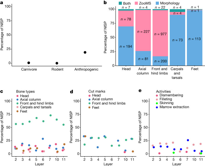
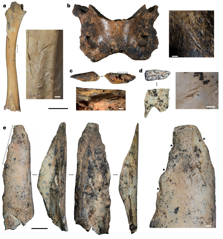
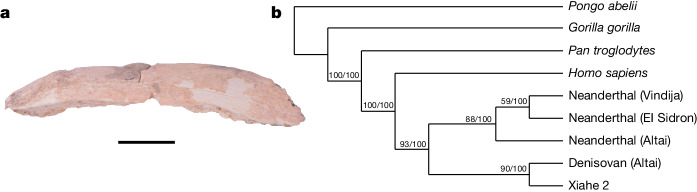
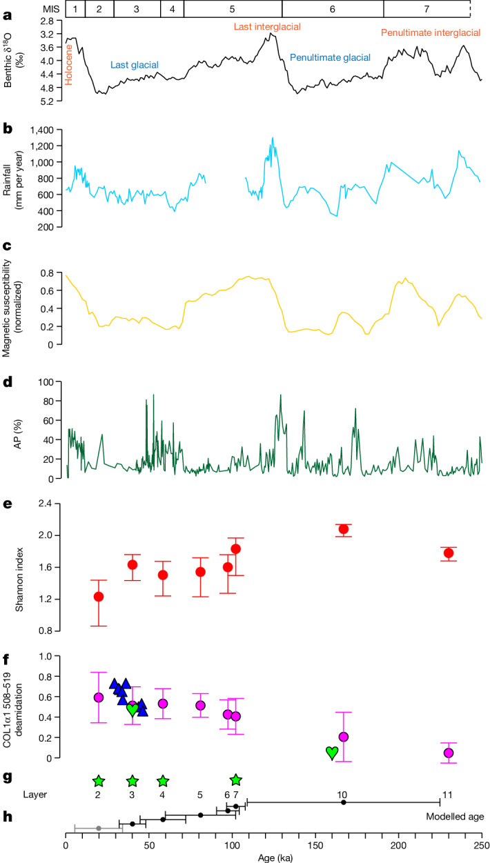
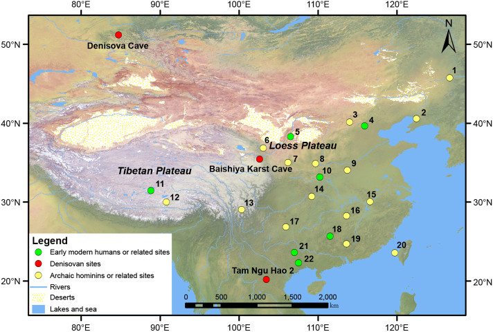
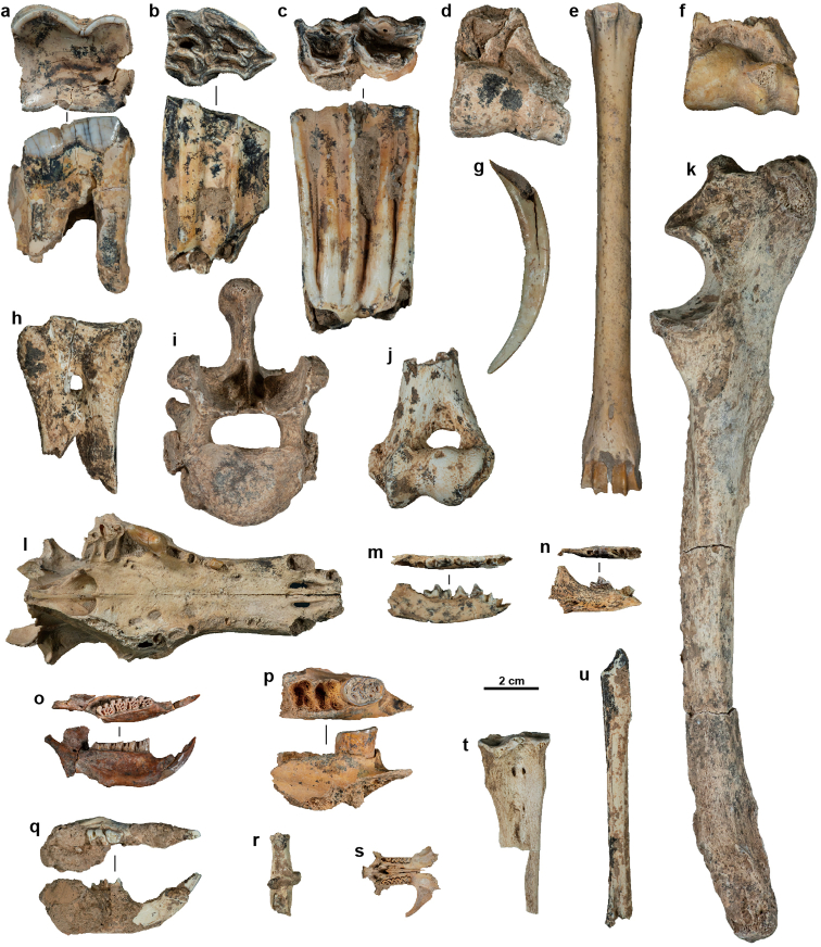
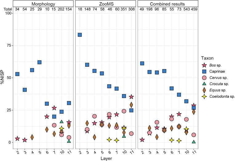
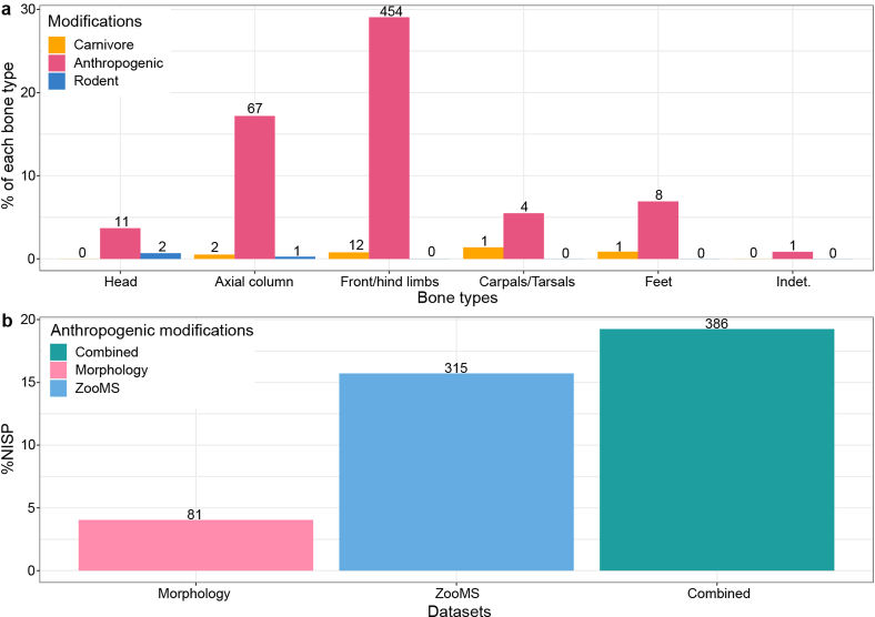
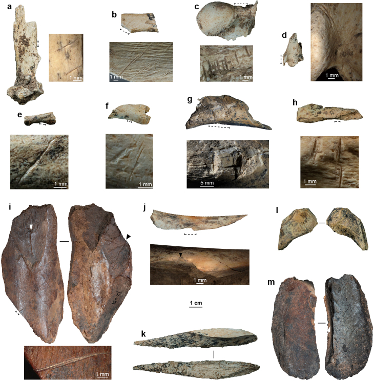
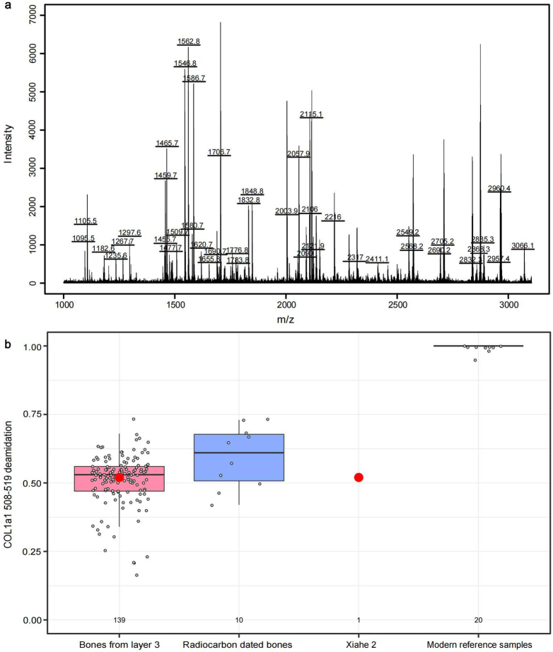
Genetic and fragmented palaeoanthropological data suggest that Denisovans were once widely distributed across eastern Eurasia^1-3. Despite limited archaeological evidence, this indicates that Denisovans were capable of adapting to a highly diverse range of environments. Here we integrate zooarchaeological and proteomic analyses of the late Middle to Late Pleistocene faunal assemblage from Baishiya Karst Cave on the Tibetan Plateau, where a Denisovan mandible and Denisovan sedimentary mitochondrial DNA were found^3,4. Using zooarchaeology by mass spectrometry, we identify a new hominin rib specimen that dates to approximately 48-32 thousand years ago (layer 3). Shotgun proteomic analysis taxonomically assigns this specimen to the Denisovan lineage, extending their presence at Baishiya Karst Cave well into the Late Pleistocene. Throughout the stratigraphic sequence, the faunal assemblage is dominated by Caprinae, together with megaherbivores, carnivores, small mammals and birds. The high proportion of anthropogenic modifications on the bone surfaces suggests that Denisovans were the primary agent of faunal accumulation. The chaîne opératoire of carcass processing indicates that animal taxa were exploited for their meat, marrow and hides, while bone was also used as raw material for the production of tools. Our results shed light on the behaviour of Denisovans and their adaptations to the diverse and fluctuating environments of the late Middle and Late Pleistocene of eastern Eurasia.

Fig. 1. Distribution of bone surface modifications and bone types at BKC.

a, Percentages of taxonomically identified specimens (n = 2,005) with carnivore, rodent or anthropogenic modifications. NISP, number of identified specimens. b, Percentages of taxonomically identified specimens within different bone types using morphology, ZooMS or both simultaneously (Supplementary Data 5). Bone types are based on morphological observations. The number shown on each bar is the corresponding NISP involved in the calculation. c, Percentages of Caprinae specimens of different bone types in each layer. d, Percentages of Caprinae specimens with cut marks on different bone types in each layer. e, Percentages of Caprinae specimens with anthropogenic modifications indicating different carcass processing activities in each layer. For a and c–e, values represent percentages of the NISP that fall into the respective categories.

Fig. 2. Examples of anthropogenically modified faunal specimens and bone tools.

a, Aquila chrysaetos right humerus (layer 4) with superficial and straight cut mark clusters, associated with the removal of feathers. b, Crocuta crocuta ultima atlas (layer 10a), with an oblique cut mark generated during disarticulation. c, Marmota sp. (ZooMS taxon ID) radius diaphysis (layer 9), with a negative conchoidal medullary flake scar (black triangle) produced by anthropogenic breakage. d, A possible retoucher (layer 11). Equus sp. right lower P2 with a set of scrape marks on its buccal surface. e, Expedient bone tool (ZooMS taxon ID: Caprinae; layer 10b). This humerus diaphysis is deliberately shaped by continuous direct percussion (indicated by black triangles in the magnified image on the right) on its cortical surface. For all panels, the enlarged images (right in a,b,d,e and bottom in c) are magnifications of the regions denoted with dotted lines in the main images. Except where noted, taxonomic identifications are from morphological analysis. Scale bars, 2 cm (a–d, main images), 1 cm (e, main image) and 1 mm (all magnified images).

Fig. 3. The Xiahe 2 specimen, a Homo sp. rib specimen discovered through ZooMS screening.

a, Photograph of the Xiahe 2 specimen. Scale bar, 1 cm. b, Phylogenetic tree for the Xiahe 2 specimen and reference proteomes. Support values at nodes are shown for the maximum likelihood and Bayesian analysis, respectively.

Fig. 4. Regional and Northern Hemisphere climate history, faunal ecology and Denisovan occupation at BKC.

a, LR04 benthic stack δ¹⁸O records. b, ¹⁰Be-based rainfall for loess samples from Baoji, northern China. c, Magnetic susceptibility (normalized) record from the Chinese Loess Plateau. d, Arboreal pollen (AP) percentages (around 600-year resolution) from the Zoige Basin, eastern margin of the Tibetan Plateau. e, Shannon index across stratigraphic units at BKC. f, Deamidation values for the peptide COL1α1 508–519 from bone specimens. The purple points and error bars represent the mean deamidation values of bones from each layer with 68.2% probability ranges. The blue triangles represent the deamidation values of individual bone specimens from layers 2–3 with radiocarbon dates (n = 9, Supplementary Data 2). The green hearts represent the deamidation values of the two Denisovan specimens (Xiahe 1 and 2). g, Stratigraphic layers and Denisovan sedimentary mtDNA. Denisovan mtDNA extracted from sediments in layers 2, 3, 4 and 7 is indicated by green stars. h, Modelled age range of each layer. The black points and the bar ranges indicate the modelled mean age and age range for each layer (Supplementary Table 2.2). The age range of layer 2 is still under evaluation, and there are currently no dates for layers 5 and 11. The indicated age range estimate for layer 5 is based on the age interval between layers 4 and 6. Detailed chronological information is available in Supplementary Information section 2.

Extended Data Fig. 1. Late Middle and Late Pleistocene sites in East Asia.

The numbers represent archaeological sites and/or hominin fossils as follows: 1. Harbin cranium; 2. Jinniushan; 3. Xujiayao; 4. Tianyuan cave; 5. Shuidonggou Locality 1 and 2; 6. Jiangjunfu 01; 7. Yangshang; 8. Dali; 9. Lingjing; 10. Huanglong Cave; 11. Nwya Devu; 12. Quesang; 13. Piluo; 14. Xinglong Cave; 15. Hualongdong; 16. Tongzi; 17. Guanyindong; 18. Fuyan Cave; 19. Maba; 20. Penghu 1; 21. Lunadong; 22. Zhirendong (Zhiren Cave). Detailed information is provided in Supplementary Data 1. Base maps generated by ArcGIS 10.7 using raster data from https://www.naturalearthdata.com/.

Extended Data Fig. 2. Photographs of faunal specimens recovered from BKC during the 2018 and 2019 excavations.

a, Coelodonta sp. left lower M1 (layer 10b). b, Equus sp. left upper P2 (layer 10b). c, Bos cf. mutus left upper M3 (layer 10). d, Ovis ammon left humerus (layer 10). e, Procapra cf. picticaudata left metacarpus (layer 2). f, Pseudois nayaur left tibia (layer 11). g, Moschus sp. right upper canine (layer 5). h, Cervus elaphus left metatarsal (layer 10). i, Panthera cf. uncia lumbar vertebra (layer 10d). j, Canis lupus left humerus (layer 11). k, Crocuta crocuta ultima left ulna (layer 10a). l, Vulpes ferrilata cranium (layer 2). m, Martes cf. foina left mandible (layer 11). n, Mustela sp. left mandible (layer 7). o, Aeretes melanopterus left mandible (layer 6). p, Hystrix cf. subcristata left mandible (layer 10a). q, Marmota himalayana left mandible (layer 10). r, Lepus oiostolus left calcaneus (layer 10c1). s, Myospalax cf. cansus cranium (layer 4). t, Aquila chrysaetos left tarsometatarsus (layer 11). u, Phasianus cf. colchicus left tibiotarsus (layer 10d). Identifications are from morphological taxonomic analysis.

Extended Data Fig. 3. Relative species composition of BKC, for selected taxa.

Proportions of selected taxa identified using morphology, ZooMS, and both combined, per layer. The total NISP for each layer is given at the top. The combined data is based on Extended Data Table 1 (n = 1,558).

Extended Data Fig. 4. Distribution of different bone surface modifications among bone specimens.

a, Percentages of bone specimens with different bone surface modifications among different bone types (indet. represents indeterminate specimens). b, Percentages of bone specimens with anthropogenic modifications identified by morphology (Supplementary Data 5A), ZooMS (Supplementary Data 5B), and both combined (Supplementary Data 5C). In a,b, the number displayed on each bar is the corresponding total NISP used in the calculation.

Extended Data Fig. 5. Examples of anthropogenic modifications on faunal specimens from BKC.

a,b, Caprinae (layer 2) (a) and class II mammal (cf. Caprinae, layer 10c) (b) vertebral neural spines, with cut marks generated during defleshing. c,d, Pseudois nayaur femoral neck (layer 3) (c) and tibia medial malleolus (layer 11) (d), with cut marks created during disarticulation. e,f, Procapra cf. picticaudata (layer 10b) (e) and Caprinae (layer 11) (f) phalanx 1, with oblique cut mark(s) generated during skinning activities. g,h, Caprinae humerus diaphysis (layer 3) (g) and femur diaphysis (layer 11; ZooMS taxon ID) (h), with two parallel chop marks related to butchering activities. i, Bos sp. humerus diaphysis (layer 9), with cut marks associated with defleshing activities. Medullary edge conchoidal flaking (black triangle) and cortical percussion surface damage (white arrow) indicate the consumption of bone marrow. j–l, Caprinae radius diaphysis (layer 7) (j) with an adhering bone flake (black triangle), and Bos sp. (ZooMS taxon ID) bone flakes (layer 10a (k) and layer 11 (l)), are indications of activities of bone marrow extraction. m, Class III/IV mammal humerus/femur diaphysis (layer 8), with evidence of burning after the diaphysis fragment was freshly broken, and showing a sequence of colour gradients from the medullary cavity to the cortex (white arrow). Except where noted, taxonomic identifications are from morphological analysis.

Extended Data Fig. 6. The Homo sp. rib specimen (Xiahe 2) identified by ZooMS.

a, MALDI-TOF MS spectrum of Xiahe 2. b, Comparison of deamidation values of Xiahe 2 with values of faunal specimens from layer 3 (n = 139, including Xiahe 2, indicated by the red point), the radiocarbon-dated bone specimens (~50–30 ka, n = 10, Supplementary Data 2) and modern reference samples (n = 20). Here, the value of 1 indicates no deamidation while the value of 0 indicates complete deamidation of the single glutamine in the marker peptide COL1α1 508–519. The box plots contain the range of the data with whiskers extending to 1.5 times the interquartile range. The boxes indicate the upper and lower quartiles, while the centre line indicates the median. All individual data points are represented by overlaid dot plots, and any data points outside the range of the box plot can be considered outliers.

Extended Data Fig. 7. Comparison of deamidation between proteomic extraction methods.

a,b, Scatter plots of COL1α1 508–519 (P1105; a) and COL1α1 435–453 (P1706; b) deamidation values for AmBic-based and acid-based extractions. The blue line and grey area indicate the mean of the loess smooth and its associated 95% confidence interval. The red line indicates a 1:1 line, where deamidation values obtained through both methods would be the same. In both cases, a high correlation is observed between the values observed for the two extraction methods (an R² of 0.93 and 0.9, respectively).

Extended Data Fig. 8. Comparison of deamidation and chronological age of the corresponding stratigraphic levels.

The distribution of COL1α1 508–519 deamidation values (P1105 68.2% probability range of each layer, indicated by the red line) in relation to the chronological age (layers 2–10; black line: age ranges of specimens with direct radiocarbon dates; blue line: age ranges of each layer, see Supplementary Table 2.2). A linear correlation (orange line) is estimated across the stratigraphy (grey shadow indicates the 95% confidence interval). Layer 11 is not included here as no direct age range is currently available. In addition, layer 10 is treated as a single, homogenous stratigraphic unit (but see Supplementary Information sections 2 and 7).

References

1. Reich, D. et al. Genetic history of an archaic hominin group from Denisova Cave in Siberia. Nature468, 1053–1060 (2010). - PMC - PubMed
1. Demeter, F. et al. A Middle Pleistocene Denisovan molar from the Annamite Chain of northern Laos. Nat. Commun.13, 2557 (2022). - PMC - PubMed
1. Chen, F. et al. A late Middle Pleistocene Denisovan mandible from the Tibetan Plateau. Nature569, 409–412 (2019). - PubMed
1. Zhang, D. et al. Denisovan DNA in Late Pleistocene sediments from Baishiya Karst Cave on the Tibetan Plateau. Science370, 584–587 (2020). - PubMed
1. Prüfer, K. et al. The complete genome sequence of a Neanderthal from the Altai Mountains. Nature505, 43–49 (2014). - PMC - PubMed
Publication types
LinkOut - more resources