. 2024 Sep;5(9):1334-1351.
doi: 10.1038/s43018-024-00787-0. Epub 2024 Jul 12.

Tumor evolution metrics predict recurrence beyond 10 years in locally advanced prostate cancer

Affiliations

Tumor evolution metrics predict recurrence beyond 10 years in locally advanced prostate cancer

Javier Fernandez-Mateos et al. Nat Cancer. 2024 Sep.

Abstract

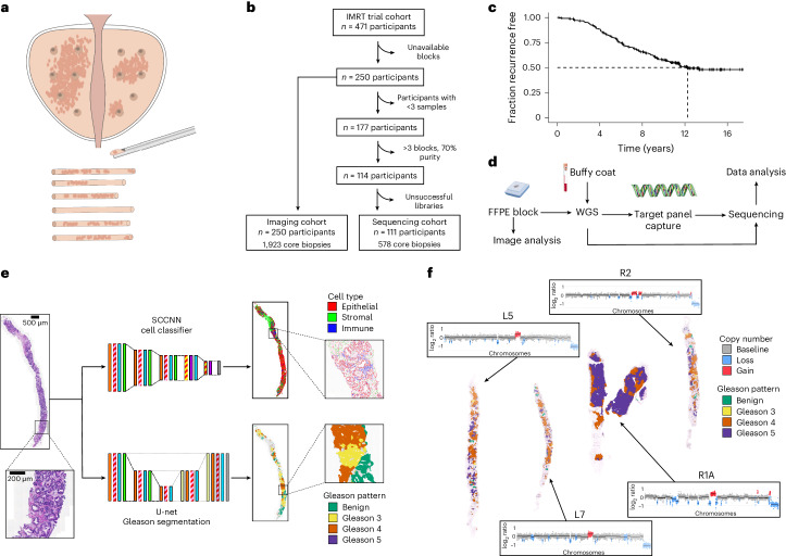
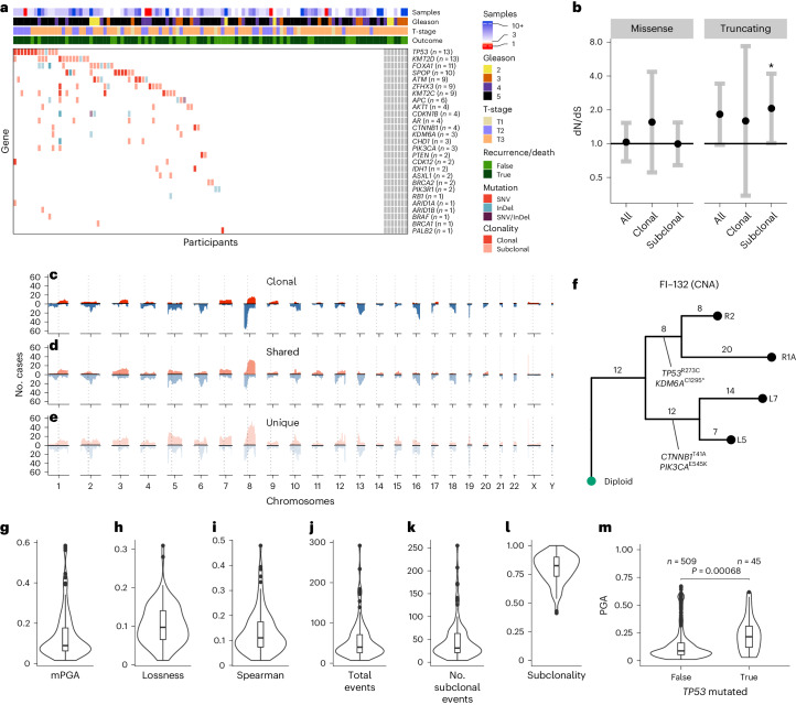
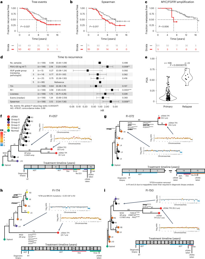
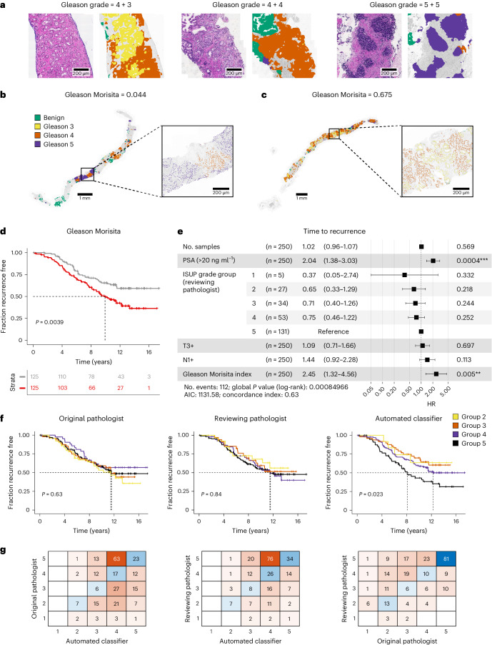
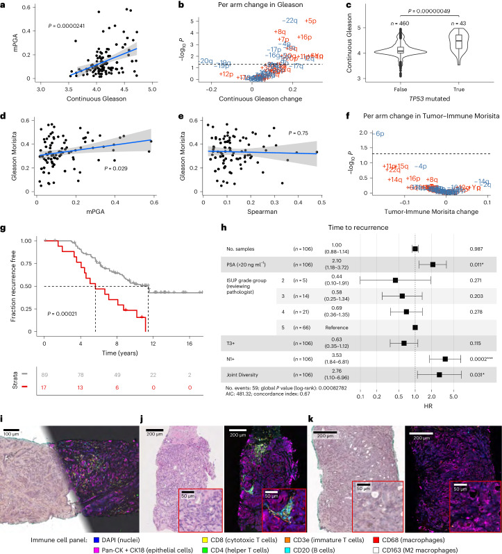
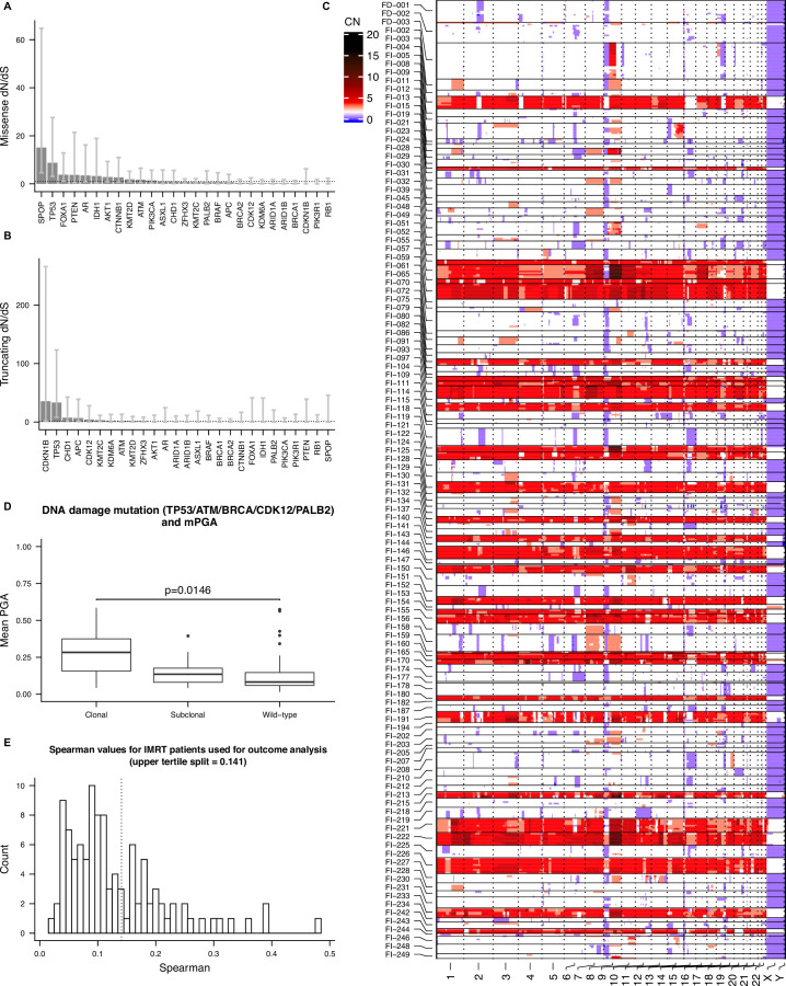
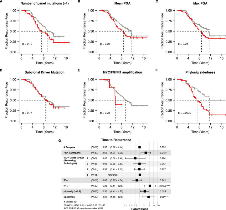
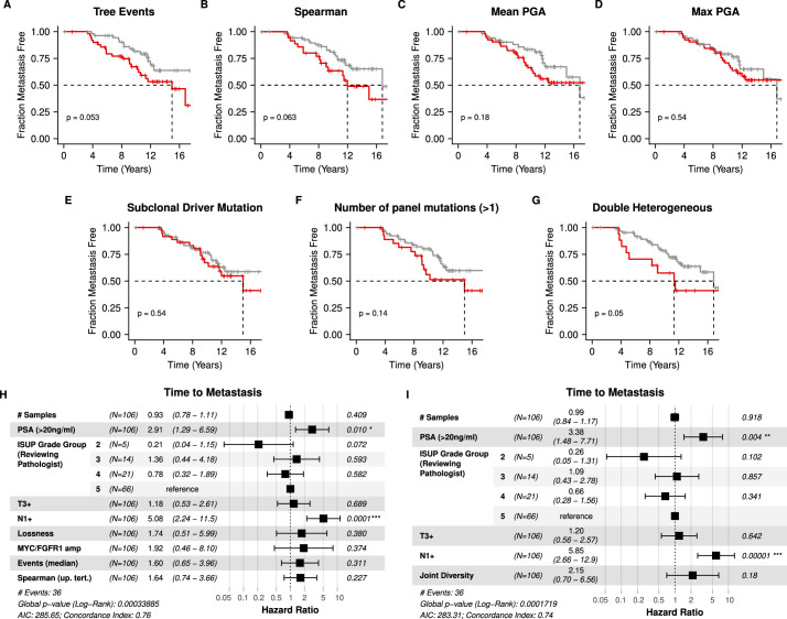
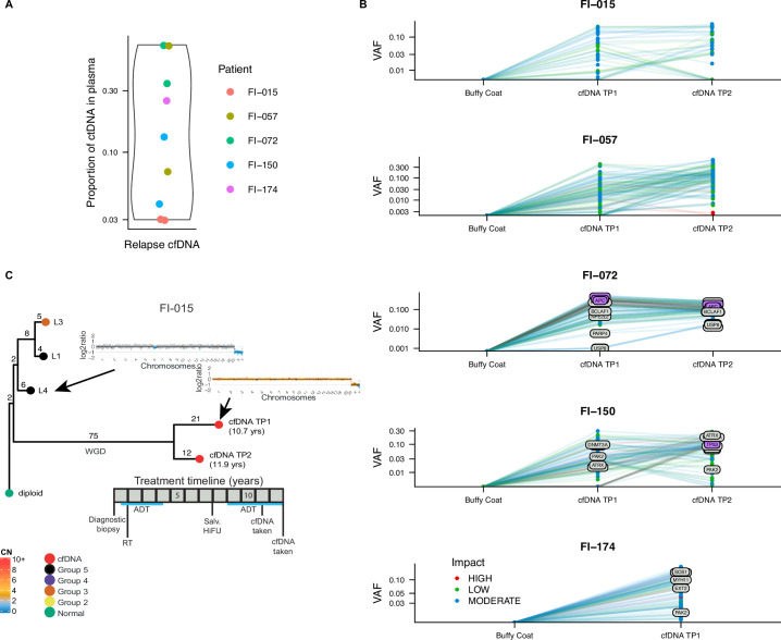
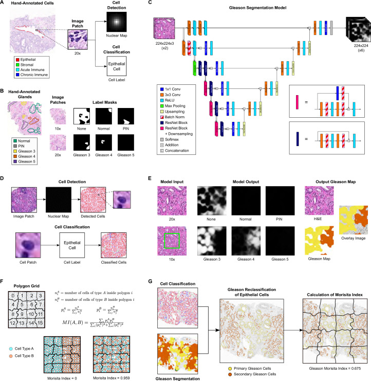
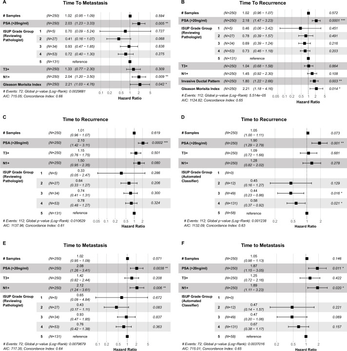
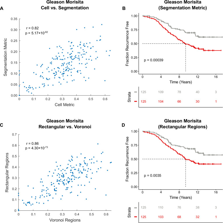
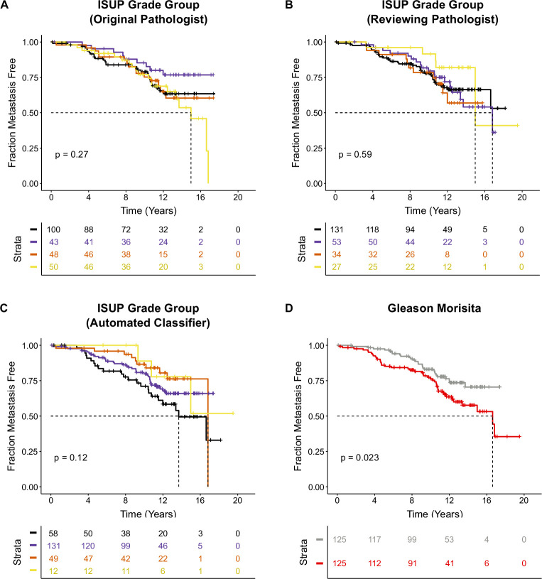
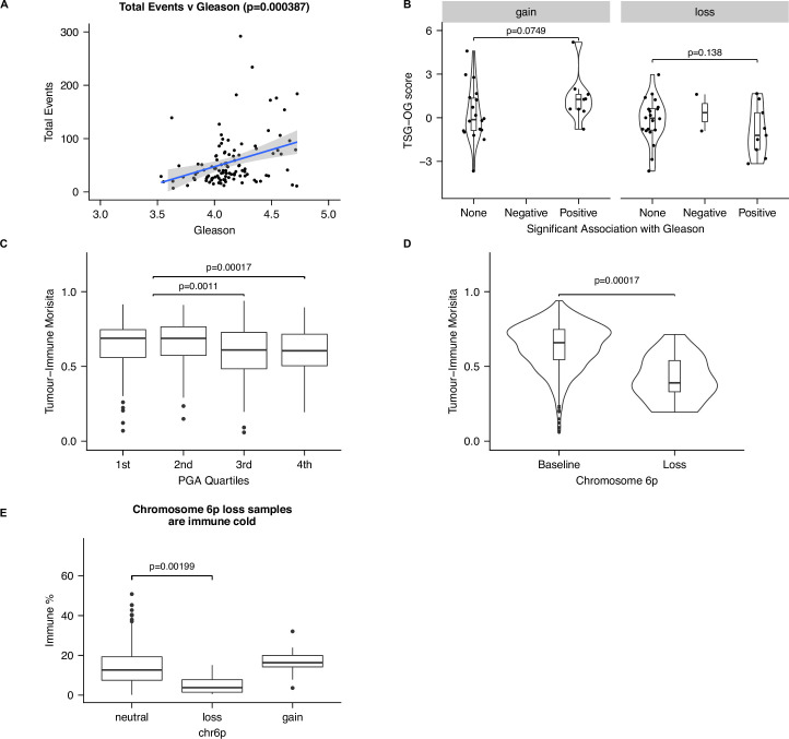
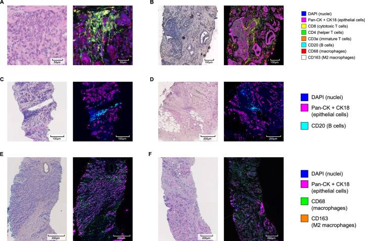
Cancer evolution lays the groundwork for predictive oncology. Testing evolutionary metrics requires quantitative measurements in controlled clinical trials. We mapped genomic intratumor heterogeneity in locally advanced prostate cancer using 642 samples from 114 individuals enrolled in clinical trials with a 12-year median follow-up. We concomitantly assessed morphological heterogeneity using deep learning in 1,923 histological sections from 250 individuals. Genetic and morphological (Gleason) diversity were independent predictors of recurrence (hazard ratio (HR) = 3.12 and 95% confidence interval (95% CI) = 1.34-7.3; HR = 2.24 and 95% CI = 1.28-3.92). Combined, they identified a group with half the median time to recurrence. Spatial segregation of clones was also an independent marker of recurrence (HR = 2.3 and 95% CI = 1.11-4.8). We identified copy number changes associated with Gleason grade and found that chromosome 6p loss correlated with reduced immune infiltration. Matched profiling of relapse, decades after diagnosis, confirmed that genomic instability is a driving force in prostate cancer progression. This study shows that combining genomics with artificial intelligence-aided histopathology leads to the identification of clinical biomarkers of evolution.

Trial registration: ClinicalTrials.gov NCT00946543.


Conflict of interest statement

D.D.’s previous employer, the Institute of Cancer Research, receives royalty income from abiraterone. D.D. receives a share of this income through the Institute of Cancer Research’s Rewards to Discoverer’s Scheme Patent (EP1933709B1), issued for a localization and stabilization device in Europe, Canada and India. D.D. receives honoraria from Janssen Pharmaceuticals. R.E. has the following conflicts of interest to declare: Honoraria from GU-ASCO, Janssen, University of Chicago, Dana Farber Cancer Institute USA as a speaker. Educational honorarium from Bayer and Ipsen, member of external expert committee to Astra Zeneca UK and Member of Active Surveillance Movember Committee. She is a member of the SAB of Our Future Health. She undertakes private practice as a sole trader at The Royal Marsden NHS Foundation Trust and 90 Sloane Street SW1X 9PQ and 280 Kings Road SW3 4NX, London, UK. The other authors declare no competing interests.

Figures

Fig. 1
Fig. 1. Study design.
a, Within the IMRT clinical trial (NCT00946543), 6–12 ultrasound-guided diagnostic needle biopsies were taken per individual for routine diagnosis and were embedded in paraffin. b, Decision tree for the imaging cohort (n = 250 individuals, n = 1,923 biopsies) and sequencing cohort (n = 111 individuals, n = 578 biopsies). The DELINEATE trial cohort was not included. c, Kaplan–Meier curve for time to recurrence in the imaging cohort (n = 250 individuals). d, Experimental workflow for FFPE biopsies and matched germline (buffy coat/normal FFPE tissue). Figure created with BioRender.com. e, Computational histopathology analysis with deep learning both for Gleason segmentation and single-cell classification on H&E sections. Sample input and output is shown for FI-115-S8; SCCNN, spatially constrained convolutional neural network. f, Example of individual FI-132, where computational Gleason segmentation and CNA genomic data were compared.
Fig. 2
Fig. 2. Genetic intratumor heterogeneity landscape of locally advanced prostate cancer.
a, Heat map representing the mutational landscape of the cohort (n = 114 participants), including number of low-pass WGS samples with detected CNAs, ISUP grade group (reviewing pathologist for IMRT participants, original specialist uropathologist S. Hazell (Royal Marsden NHS Foundation Trust) for DELINEATE, where participants were not reviewed), T-stage and recurrence/death status. Mutations are colored and shaded by their type (SNV and insertion/deletion (InDel)) and clonality status (clonal/subclonal). b, dN/dS analysis of all mutations using dNdScv for missense and truncating mutations shows subclonal truncating mutations to be under positive selection. Clonal and subclonal mutations were taken only from participants with three or more targeted sequencing samples (all n = 107 participants, clonal/subclonal n = 98 participants). Intervals represent 95% CI, and the centers represent the maximum likelihood estimate. ce, CNA landscape of prostate cancer defined by phylogenetic status per case. Gains (red) and losses (blue) are represented relative to ploidy of the samples (n = 111 participants). f, An example of MEDICC2-inferred CNA phylogeny in FI-132 with manually annotated driver SNVs. gl, Genomic metrics of genomic instability and heterogeneity were calculated before outcome unblinding (n = 109 participants, sequencing cohort participants with three or more samples with a PGA of ≥0.01). m, TP53-mutant samples presented with significantly higher PGA (linear mixed effects model, two-sided t-test on gradient, s.e. = 0.02, d.f. = 552, t = 3.4, samples with a PGA of ≥0.01, n = 554 samples). Box plots show the center line as the median and box limits as upper and lower quartiles. Whiskers extend no further than 1.5× the interquartile range past the box limits, and points represent outliers. Source data
Fig. 3
Fig. 3. Spatial genetic diversity and phylogenetic events predict recurrence.
a,b, Total phylogenetic tree events (two-sided log-rank test, χ2 = 4.9, d.f. = 1; a) and the Spearman metric (two-sided log-rank test, χ2 = 5.7, d.f. = 1; b) predict earlier time to recurrence (n = 106 participants, sequencing cohort IMRT participants with three or more samples with a PGA of ≥0.01). c, Amplification in MYC and/or FGFR1 (coamplified in one participant) predicts earlier time to metastasis (two-sided log-rank test, χ2 = 7.5, d.f. = 1, n = 106 participants). d, Cox proportional hazards (CPH) model of time to recurrence using clinical covariates and number of low-pass WGS samples with CNAs. Three metrics significant in a univariate CPH model (P < 0.1) are also included in the model (natural log of lossness, total phylogenetic events split by median value and Spearman). The forest plot shows 95% CI of HRs and the covariate P values, derived from a Wald test (n = 106 participants, *P < 0.05, **P < 0.01, ***P < 0.001). HRs for lossness and Spearman represent the increase in hazard between their 5th and 95th percentile values (within the sequencing cohort). e, mPGA per participant in primary samples (n = 109 participants) compared to the mPGA of individual relapse samples (n = 9 samples, two-sided Mann–Whitney U-test, W = 962). fi, Phylogenetic analysis of primary and relapse samples (cfDNA) taken at recurrence. Tips of tumor nodes represent either the automated classifier ISUP grade group (primary diagnostic biopsies) or a cfDNA sample (red). Time since the diagnostic biopsy is labeled next to the cfDNA nodes in years (yrs). Representative copy number profiles are shown for a single cfDNA sample and the primary diagnostic biopsy that is most related to the cfDNA. Edges are labeled with phylogenetic events plus specific CNA events (for example, whole-genome duplication (WGD) or gene amplification (amp)) or detected point mutations. Genes present in the diagnostic biopsy panel are highlighted in bold and may be detected in both the primary and relapse samples. Genes not in bold are only detectable in the relapse samples and may also be present in the diagnostic biopsies. Below each tree, the timeline shows treatment history. Each event is rounded to the nearest 6 months. Each square represents a year. Treatment descriptions are written in shorthand; Abi, abiraterone acetate; Cab, cabazitaxel; CN, copy number; Dex, dexamethasone; Doce, docetaxel; Enza, enzalutamide; Ra-223, radium-223; RT, radiotherapy; Salv. HiFU, salvage high-intensity focused ultrasound; VAF, variant allele frequency. Source data
Fig. 4
Fig. 4. Morphological spatial heterogeneity with deep learning-based Gleason grading.
a, Example output from the automated Gleason classifier, with primary and secondary pattern assessment. b,c, Examples of the Gleason Morisita assessment. Cells identified as epithelial cells by the cell classifier are subdivided into Gleason grades using the region’s automated Gleason segmentation. Regions with high segregation of patterns (b) will be assigned a low Gleason Morisita index, whereas regions with high mixing between Gleason grades (c) will be assigned a high Gleason Morisita index. d, Participants with greater within-section heterogeneity of Gleason pattern, as assessed by Gleason Morisita index, are associated with a shorter time to recurrence (two-sided log-rank test, χ2 = 8.33, d.f. = 1, P = 0.0039; imaging cohort, n = 250 participants). e, CPH model of time to recurrence using clinical covariates and the Gleason Morisita index (imaging cohort, n = 250 participants, *P < 0.05, **P < 0.01, ***P < 0.001). The forest plot shows 95% CI of HRs and the covariate P values, derived from a Wald test. HR for the Gleason Morisita index represents the increase in hazard between the 5th and 95th percentile values (within the imaging cohort). f, ISUP grade group as a predictor of time to recurrence. A comparison is shown for the grade groups assessed by the original reporting pathologist, the reviewing pathologist for the trial and the automated classifier (imaging cohort, n = 250 participants). Grade groups are calculated from the assessed primary and secondary patterns, according to the 2014 ISUP criteria. Only the automated Gleason assessment was able to stratify the participants by time to recurrence (two-sided log-rank test, χ2 = 9.52, d.f. = 3, P = 0.023). g, Confusion matrices showing the pairwise agreement of the ISUP grade groups reported by the original reporting pathologist, the reviewing pathologist for the trial and the automated classifier (imaging cohort, n = 250 participants). Source data
Fig. 5
Fig. 5. Combining genetic and morphological measurements.
a, mPGA is associated with higher continuous Gleason (n = 106 participants, IMRT participants with three or more samples with a PGA of ≥0.01, linear model, two-sided t-test on gradient, estimate = 0.19, s.e. = 0.04, t = 4.4, d.f. = 104). Shaded area represents 95% CI in all scatter plots. b, Twenty-four chromosome arm changes are associated with a change in continuous Gleason (gains are displayed in red, and losses are displayed in blue; n = 62 chromosome arm changes, P values were adjusted using the Benjamini–Hochberg method and are derived from two-sided t-tests on gradient per arm linear mixed effects model; continuous Gleason change derived from gradient estimate). c, The TP53 mutation is associated with higher continuous Gleason (linear mixed effects model, two-sided t-test on gradient, s.e. = 0.06, d.f. = 371, t = 5.1, n = 503 samples). Box plots show center lines as the median and box limits as upper and lower quartiles. Whiskers extend no further than 1.5× interquartile range past the box limits, and points represent outliers. d,e, mPGA (linear model, two-sided t-test on gradient, estimate = 0.23, s.e. = 0.103, t = 2.2, d.f. = 85; d), but not Spearman (estimate = −0.05, s.e. = 0.15, t = −0.3, d.f. = 85; e), is associated with increased mixing of Gleason grades (n = 87 participants, sequencing cohort omitting participants with a Gleason Morisita equal to 0, that is, a homogenous Gleason grade). f, Chromosome 6p loss is uniquely associated with a reduction in Tumor-Immune Morisita (changes are colored and P values were adjusted and derived as in b; n = 62 chromosome arm changes). Samples in b, c and f have a PGA of ≥0.01. g, The most genetically and morphologically heterogeneous tumors are associated with shorter time to recurrence (two-sided log-rank test, χ2 = 13.7, d.f. = 1, n = 106 participants). h, The Joint Diversity metric shows significant association with greater risk of recurrence in a CPH model with clinical covariates. The forest plot shows 95% CI of HRs, and the covariate P values are derived from a Wald test. The HR for Joint Diversity represents the increase in hazard between the 5th and 95th percentile values (within the sequencing cohort, n = 106 participants, *P < 0.05, **P < 0.01, ***P < 0.001). i, Multiplex immunohistochemistry and H&E staining was performed on the same section. Immunohistochemistry experiments were run once following optimization and validation. j, Example of an immune-hot region on matched H&E (left) and multiplex immunohistochemistry (right) images. k, Example of an immune-cold region on matched H&E (left) and multiplex immunohistochemistry (right) images. Source data
Extended Data Fig. 1
Extended Data Fig. 1. Genomic analysis of locally-advanced prostate cancer.
(A) Estimates of per-gene dN/dS for missense mutations only. dN/dS maximum likelihood estimates are calculated per gene by dNdScv. Intervals represent 95% confidence level, the bars represent the maximum likelihood estimate and dotted line represents dNdS = 1 (neutral). Missense mutations are positively selected in SPOP, TP53 and FOXA1 as the lower bounds of the intervals are greater than 1. (B) Estimates of per-gene dN/dS for truncating mutations only. Intervals represent 95% confidence level, the bars represent the maximum likelihood estimate and dotted line represents dNdS = 1 (neutral). Truncating mutations are positively selected in CDKN1B and TP53. Number of mutation types per gene are provided in source material. (C) A heatmap of per sample absolute copy number calls. Chromosomes are represented on the x-axis and samples are grouped by participant on the y-axis, separated by lines (n = 609 samples, n = 114 participants). Copy numbers are not normalised relative to baseline ploidy. (D) DNA damage mutations versus mean PGA. Boxplots represent mean PGA (mPGA) separated based on the clonality of mutations involved in DNA damage response (TP53, ATM, BRCA1/2, CDK12, PALB2). The status is considered clonal if any of the mutations are detected in all samples. mPGA is significantly higher in participants with a clonal DNA damage mutation compared to participants with no DNA damage mutations (2-sided t-test, standard error = 0.055, d.f. = 10.1, t = 2.94). Mutations are split into clonal (n = 10 participants), subclonal (n = 13 participants) and wild-type (n = 75 participants). Boxplots show centre line as median, box limits as upper and lower quartiles, whiskers extend no further than 1.5x interquartile range past the box limits and points represent outliers. (E) Distribution of Spearman values for cohort (n = 106 participants) used for outcome analysis displays a long tail of high values that are discriminated by a threshold of the upper tertile (dotted line). Source data
Extended Data Fig. 2
Extended Data Fig. 2. Time to recurrence analysis of genomic metrics.
(A) Participants are split between those with >1 mutated gene on the panel (red, n = 29 participants) and those with 1 or 0 (grey, n = 66 participants). This threshold produced the best split of the data in time to recurrence analysis. (B) Participants are split by the median mPGA. Participants with high mPGA (red, n = 53 participants) do not have significantly shorter time to recurrence than those with low mPGA (grey, n = 53 participants). (C) Participants are split by the median max PGA. Participants with high max PGA (red, n = 53 participants) do not have significantly shorter time to recurrence than those with low max PGA (grey, n = 53 participants). (D) Participants are split between those that had a subclonal mutation on the driver gene panel (red, n = 38 participants) and those without (grey, n = 57 participants). KMT2C and KMT2D were excluded from this analysis. (E) Participant with an amplification in MYC and/or FGFR1 (red, n = 5 participants) did not have significantly different time to recurrence than those with an absence of either amplification (grey, n = 101 participants). All p values are calculated using a log-rank test. (F) Participants with strong sidedness (greater clustering of right and left regions across the MEDICC2 tree, lambda > 0.8, red, n = 36 participants) show a significantly shorter time to recurrence (log-rank test) than the remaining participants for which phylogenetic signal analysis was possible (grey, n = 31 participants). (G) Cox proportional hazards (CPH) model of time to recurrence using clinical co-variates, phylosig sidedness classification and Spearman (n = 67 participants). Forest plot shows 95% confidence interval of hazard ratios, and the covariate P values, derived from a Wald test (*P < 0.05, ** P < 0.01, ***P < 0.001). Hazard ratio for Spearman represents the increase in hazard between the 5th and 95th percentile values (within the Sequencing Cohort). Source data
Extended Data Fig. 3
Extended Data Fig. 3. Time to metastasis analysis of genomic metrics.
(A) Participants with a high number of events (greater than median, red, n = 50 participants) did not have a significantly shorter time to metastasis than those with fewer events (grey, n = 56 participants). (B) Participants split by the upper tertile of the Spearman metric (red, n = 35 participants) and the lower two tertiles (grey, n = 71 participants). (C) Participants are split by the median mPGA. Participants with high mPGA (red, n = 53 participants) do not have significantly shorter time to metastasis than those with low mPGA (grey, n = 53 participants). (D) Participants are split by the median max PGA. Participants with high max PGA (red, n = 53 participants) do not have significantly shorter time to metastasis than those with low max PGA (grey, n = 53 participants). (E) Participants are split between those that had a subclonal mutation on the driver gene panel (red, n = 38 participants) and those without (grey, n = 57 participants). KMT2C and KMT2D were excluded from this analysis. (F) Participants are split between those with >1 mutated gene on the panel (red, n = 29 participants) and those with 1 or 0 (grey, n = 66 participants). (G) Participants split equally to Fig. 5G. Double heterogeneous participants (red, n = 17 participants) had a significantly shorter time to metastasis than the rest (grey, n = 89 participants, P = 0.0497). P values are calculated using a log-rank test. (H) CPH model, using clinical co-variates and genomic metrics with p < 0.1 in a univariate CPH model, for time to metastasis. (I) Cox proportional hazards (CPH) model, using clinical co-variates and Joint Diversity metric, for time to metastasis. Forest plots show 95% confidence interval of hazard ratios, and the covariate P values, derived from a Wald test (*P < 0.05, **P < 0.01, ***P < 0.001). Hazard ratios for Lossness and Joint Diversity represent the increase in hazard between their 5th and 95th percentile values (within the Sequencing Cohort). Source data
Extended Data Fig. 4
Extended Data Fig. 4. Time series genomic analysis of ctDNA samples at recurrence.
(A) Distribution of the proportion of ctDNA in plasma across 9 cfDNA samples in 5 participants within fragments between 90 and 150 bp in size. (B) Trajectories of changes in variant allele frequency (VAF) across cfDNA timepoints for 5 participants. Lines and dots represent synonymous and non-synonymous mutations derived from whole exome sequencing and their impact as determined by VEP. Buffy coats represent control samples. Mutations are labelled if they belong to the targeted panel used for the primary samples (purple) or if they overlap with the IntOGen (www.intogen.org) pan-cancer driver list (grey) (n = 35 mutations, n = 100 mutations, n = 111 mutations, n = 94 mutations, n = 84 mutations, top to bottom). (C) MEDICC2 copy number alteration phylogenetic tree for FI-015 with cfDNA and primary diagnostic biopsy samples. Tips of nodes represent either the ISUP Grade group (primary diagnostic biopsies) or if the sample is a cfDNA sample (red). Time since the diagnostic biopsy is labelled next to the cfDNA nodes in years (yrs). Representative copy number profiles are shown for a single cfDNA sample and the primary diagnostic biopsy that is most related to the cfDNA. Edges are labelled with copy number alteration events (for example, WGD, whole genome duplication). Below the tree the timeline shows treatment history. Each event is rounded to the nearest 6 months. Each square represents a year. Treatment descriptions are written in shorthand (ADT = Androgen Deprivation Therapy, RT = Radiotherapy, Salv. HiFU = Salvage High-intensity Focused Ultrasound). Source data
Extended Data Fig. 5
Extended Data Fig. 5. Digital Pathology methods outline.
(A) Cell detection and classification model training. Cells are manually annotated onto the slide. For cell detection, annotated cells are converted into an input image patch and an output nuclear probability map. For cell classification, annotated cells are converted into an input image patch and a cell label. (B) Gleason segmentation model training. Glandular regions are manually annotated onto the slide, which are converted into input images patches and output segmentation masks. Input images are at 20x and 10x magnification, each centred at the same point. Output masks represent the segmentation of each class on the 20x input image. (C) Neural network architecture for Gleason segmentation model. Layers are represented by rectangles, colour coded by their type. Arrows indicate connections between layers. Dimensions of the output neurons are listed for each layer. (D) Outline of cell detection and classification. From an input image patch, the cell detector outputs a cell probability map, which is converted into cell detections. For each detected nuclei, an image patch is extracted. This is processed by the cell classifier, producing a label for the cell. (E) Outline of Gleason segmentation. As input, the network receives 20x and 10x images (20x image region is indicated on the 10x image in green). The network outputs probability maps for each label, corresponding to the 20x image. An output Gleason map is generated from the probability maps. (F) Outline of cellular Morisita index. Metric estimates the degree of mixing between two cell populations. Visual examples are shown for both high segregation and high mixing of cells. (G) Calculation of Gleason Morisita index. Epithelial cells are reclassified by the Gleason grade of their associated gland. The Gleason Morisita index is computed between the epithelial cells of the section’s primary and secondary Gleason patterns. For further details see ‘Computational Analysis’ supplementary note.
Extended Data Fig. 6
Extended Data Fig. 6. Supplementary Cox proportional hazards (CPH) models from Digital Pathology analysis.
(A) Time to metastasis using clinical co-variates and Gleason Morisita index (Imaging Cohort, n = 250 participants). Increased Gleason Morisita index is significant associated with shorter time to recurrence (p < 0.05), in line with what is seen in time to recurrence (Fig. 4E). Hazard ratio for Gleason Morisita index represents the increase in hazard between the 5th and 95th percentile values (within the Imaging Cohort). (B) Time to recurrence using clinical co-variates, presence of Invasive Ductal Pattern, and Gleason Morisita index (Imaging Cohort, n = 250 participants). Both Gleason Morisita index and Invasive Ductal Pattern are independently significant predictors of risk of patient recurrence (p < 0.05). Presence of Invasive Ductal Pattern was identified at a per-patient level by Reviewing Pathologist. Hazard ratio for Gleason Morisita index represents the increase in hazard between the 5th and 95th percentile values (within the Imaging Cohort). (C) Time to recurrence, including clinical covariates and Reviewing Pathologist’s grade grouping (Imaging Cohort, n = 250 participants). Model hazard ratios suggest a decreasing risk of recurrence as grade group decreases, with respect to reference group 5, albeit without significance. (D) Time to recurrence, including clinical covariates and grade grouping from automated classifier (Imaging Cohort, n = 250 participants). Grade groups 3 and 4 show significantly lower risk of recurrence (P = 0.0164 and P = 0.0214, respectively) compared to reference group 5. (E) Time to metastasis, including clinical covariates and Reviewing Pathologist’s grade grouping (Imaging Cohort, n = 250 participants). There is no clear trend for grade group. (F) Cox model of time to metastasis, including clinical covariates and grade grouping from automated classifier (Imaging Cohort, n = 250 participants). Model hazard ratios suggest a decreasing risk of metastasis from groups 3–5, albeit without significance. All forest plots show 95% confidence interval of hazard ratios and the covariate P values, derived from a Wald test (*P < 0.05, **P < 0.01, ***P < 0.001). Source data
Extended Data Fig. 7
Extended Data Fig. 7. Evaluation of the robustness of Gleason Morisita index.
To evaluate the robustness of Gleason Morisita index, two comparisons are made: balance of epithelial cells vs. balance of segmented pixels (A, B), and Voronoi sub-regions vs. rectangular subregions (C, D). (A) Scatter plot comparing patient-level Gleason Morisita indices from the cell and segmentation-based metrics. The two metrics are well correlated, with a Pearson correlation of 0.82 (Imaging Cohort, n = 250 participants, d.f. = 248, P = 5.17 × 10−62). (B) KM curve of time to recurrence for segmentation-based Gleason Morisita index, split by median. Segmentation-based metric is also a significant predictor of time to recurrence (Imaging Cohort, n = 250 participants, two-sided log-rank test, χ2 = 10.43, d.f. = 1, P = 0.00039), with the pattern of survival closely resembling that of the cell-based metric (Fig. 4D). (C) Scatter plot comparing patient-level Gleason Morisita indices from the Voronoi and rectangular regions. The two metrics are well correlated, with a Pearson correlation of 0.86 (Imaging Cohort, n = 250 participants, d.f. = 248, P = 4.3 × 10−73). (D) KM curve of time to recurrence for Gleason Morisita index from rectangular regions, split by median. Rectangular region metric is also a significant predictor of time to recurrence (Imaging Cohort, n = 250 participants, two-sided log-rank test, χ2 = 5.94, d.f. = 1, P = 0.0035), with the pattern of survival closely resembling that of the Voronoi region metric (Fig. 4D). Source data
Extended Data Fig. 8
Extended Data Fig. 8. Univariate KM curves of time to metastasis for Gleason grading and Gleason Morisita.
(A) Gleason grading from original reporting pathologists (Imaging Cohort, n = 250 participants, two-sided log-rank test, χ2 = 7.05, d.f. = 3, P = 0.27). (B) Gleason grading from reviewing pathologist (Imaging Cohort, n = 250 participants, two-sided log-rank test, χ2 = 2.28, d.f. = 3, P = 0.59). (C) Gleason grading from automated classifier (Imaging Cohort, n = 250 participants, two-sided log-rank test, χ2 = 5.83, d.f. = 3, P = 0.12). (D) Gleason Morisita index, split by median. Only Gleason Morisita index shows a significant difference in time to metastasis (Imaging Cohort, n = 250 participants, two-sided log-rank test, χ2 = 5.17, d.f. = 1, P = 0.023). Source data
Extended Data Fig. 9
Extended Data Fig. 9. Associations of genomic markers with Digital Pathology analysis.
(A) Comparison of continuous Gleason values (n = 106 participants) and the total number of phylogenetic CNA events. Trees with more events had a greater continuous Gleason value (linear model, 2-sided t-test on gradient, estimate = 63.7, standard error = 17.36, t = 3.67, d.f. = 104). Shaded area represents 95% confidence interval. (B) Association of TSG-OG score and the correlation of chromosome arm changes with continuous Gleason. Each data point represents the TSG-OG score (higher indicates more oncogene rich, lower indicates more tumour suppressor rich, Davoli et al.) for a chromosome arm. Arms are then categorised according to if the test compared a gain or loss of the arm to the baseline level. Values are further categorised by whether the arm gain or loss is associated with no change in continuous Gleason (None, gain n = 18 arms, loss n = 20 arms), a reduction in continuous Gleason (Negative, loss n = 2 arms) or an increase in continuous Gleason (Positive, gain n = 9 arms, loss n = 9 arms). P-values are derived from one sided t-tests (gain, standard error = 0.71, d.f. = 18.6, t = −1.5; loss, standard error = 0.67, d.f. = 14, t = 1.1). Boxplots show centre line as median, box limits as upper and lower quartiles, whiskers extend no further than 1.5x interquartile range past the box limits and points represent outliers. (C) Samples present in the upper two quartiles (n = 138 samples for each quartile) of PGA values are associated with reduced Tumour-Immune Morisita when separately compared to the first two quartiles combined (2-sided Mann-Whitney U tests, W = 15312, 3rd Quartile; W = 14728, 4th Quartile). Boxplots show centre line as median, box limits as upper and lower quartiles, whiskers extend no further than 1.5x interquartile range past the box limits and points represent outliers. (D) Chromosome 6p loss (n = 20 samples) is associated with a lower Tumour-Immune Morisita compared to those with baseline CN (n = 516 samples). Linear mixed effects model, 2-sided t-test on gradient, estimate = −0.16, standard error = 0.04, d.f. = 458, t = −3.8. P-value is not adjusted for multiple hypothesis testing. Boxplots show centre line as median, box limits as upper and lower quartiles, whiskers extend no further than 1.5x interquartile range past the box limits and points represent outliers. (E) Chromosome 6p loss samples (n = 20 samples) have a significantly lower percentage of immune cells than those with a baseline chromosome 6p copy number (n = 516 samples, linear mixed effects model, 2-sided t-test on gradient, standard error = 2.01, d.f. = 525, t = −3.1). 16 samples had a gain in chromosome 6p. Boxplots show centre line as median, box limits as upper and lower quartiles, whiskers extend no further than 1.5x interquartile range past the box limits and points represent outliers. Source data
Extended Data Fig. 10
Extended Data Fig. 10. Supplementary examples of immune profiles in the multiplex immunohistochemistry cohort.
Each image pair shows the expression of immunofluorescence markers (right), acquired by Phenocycler Fusion, with the matched region from H&E staining (left). (A, B) Examples of immune hot regions. (C, D) Examples of regions abundant for CD20 (cyan). (E, F) Examples of regions abundant for CD68 (green). CD163 (orange) is rarely seen, suggesting that these are likely to be solely M1 macrophages. Immunohistochemistry experiments were run once following optimisation and validation.

Similar articles

Cited by

References

    1. van Leenders, G. J. L. H. et al. The 2019 International Society of Urological Pathology (ISUP) Consensus Conference on Grading of Prostatic Carcinoma. Am. J. Surg. Pathol.44, e87–e99 (2020). - PMC - PubMed
    1. Dess, R. T. et al. Development and validation of a clinical prognostic stage group system for nonmetastatic prostate cancer using disease-specific mortality results from the International Staging Collaboration for Cancer of the Prostate. JAMA Oncol.6, 1912–1920 (2020). - PMC - PubMed
    1. Lorent, M. et al. Meta-analysis of predictive models to assess the clinical validity and utility for patient-centered medical decision making: application to the CAncer of the Prostate Risk Assessment (CAPRA). BMC Med. Inform. Decis. Mak.19, 2 (2019). - PMC - PubMed
    1. Zelic, R. et al. Predicting prostate cancer death with different pretreatment risk stratification tools: a head-to-head comparison in a nationwide cohort study. Eur. Urol.77, 180–188 (2020). - PubMed
    1. Taylor, B. S. et al. Integrative genomic profiling of human prostate cancer. Cancer Cell18, 11–22 (2010). - PMC - PubMed

Substances

Associated data