Keypoint-MoSeq: parsing behavior by linking point tracking to pose dynamics

Abstract

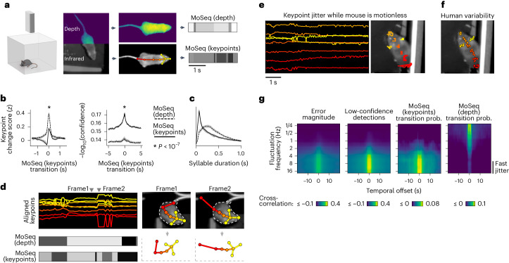
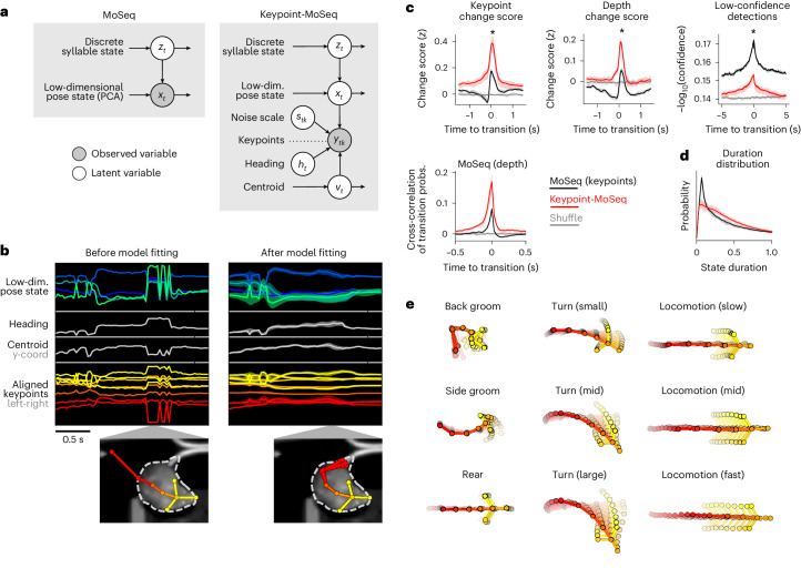
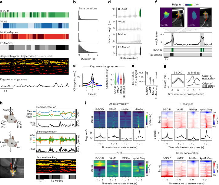
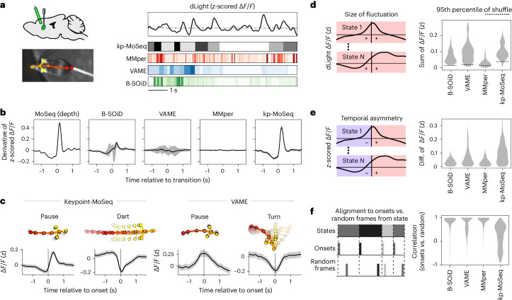
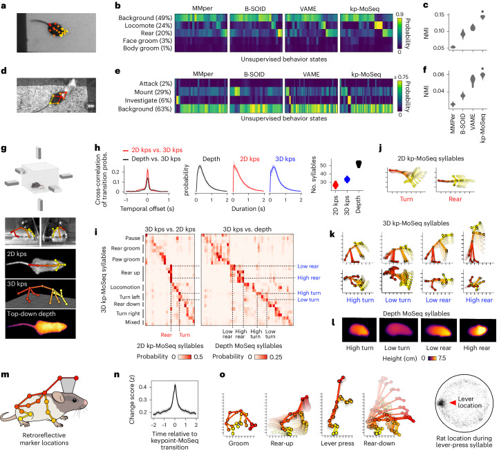
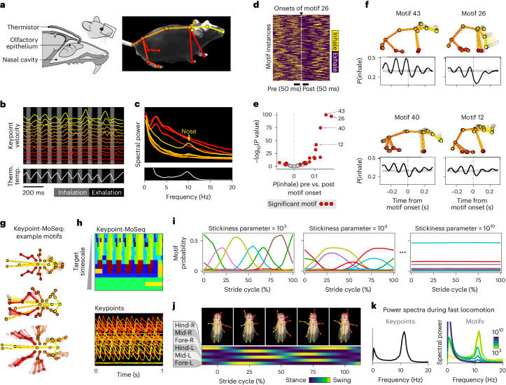
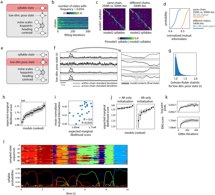
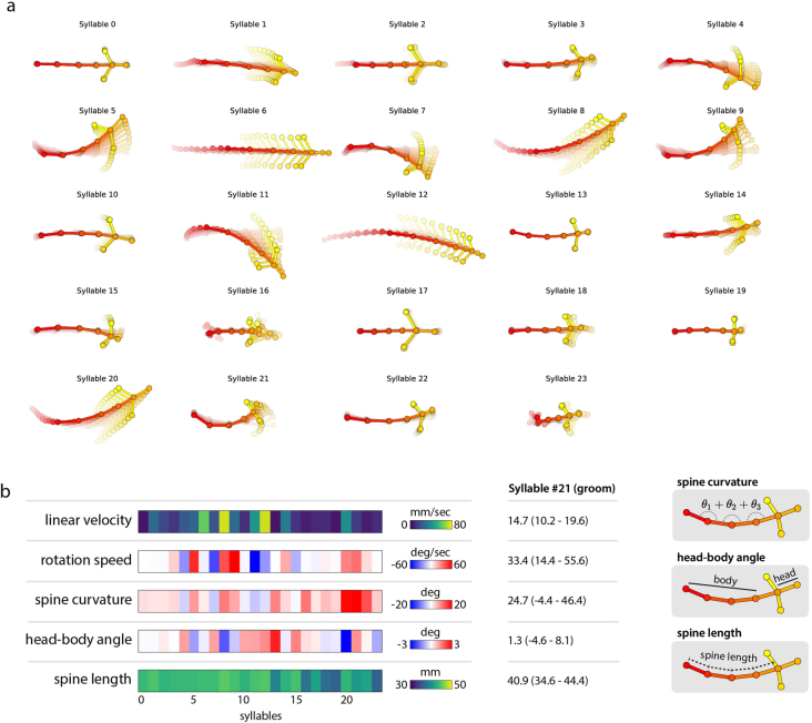
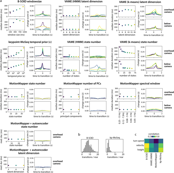
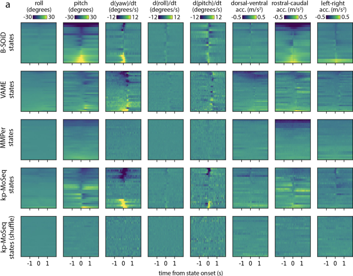
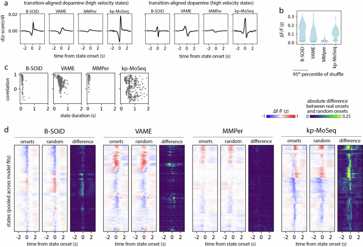
Keypoint tracking algorithms can flexibly quantify animal movement from videos obtained in a wide variety of settings. However, it remains unclear how to parse continuous keypoint data into discrete actions. This challenge is particularly acute because keypoint data are susceptible to high-frequency jitter that clustering algorithms can mistake for transitions between actions. Here we present keypoint-MoSeq, a machine learning-based platform for identifying behavioral modules ('syllables') from keypoint data without human supervision. Keypoint-MoSeq uses a generative model to distinguish keypoint noise from behavior, enabling it to identify syllables whose boundaries correspond to natural sub-second discontinuities in pose dynamics. Keypoint-MoSeq outperforms commonly used alternative clustering methods at identifying these transitions, at capturing correlations between neural activity and behavior and at classifying either solitary or social behaviors in accordance with human annotations. Keypoint-MoSeq also works in multiple species and generalizes beyond the syllable timescale, identifying fast sniff-aligned movements in mice and a spectrum of oscillatory behaviors in fruit flies. Keypoint-MoSeq, therefore, renders accessible the modular structure of behavior through standard video recordings.

Fig. 1. Keypoint trajectories exhibit sub-second structure.

a, Left: simultaneous depth and 2D infrared (IR) recording setup. Middle: pose representations using the depth data (top) or IR (bottom, tracked keypoints indicated). Right: Example syllable sequences from MoSeq applied to depth data (referred to as ‘MoSeq (depth)’) or to keypoint data (referred to as ‘MoSeq (keypoints)’). Figure created with SciDraw under a CC BY 4.0 license. b, Keypoint change scores or low-confidence detection scores, relative to the onset of MoSeq transitions (x axis) derived from either depth (gray) or keypoint (black) data. Differences in each case were significant (P = 2 × 10⁻⁷ over N = 20 model fits, Mann–Whitney U test; plots show mean and range across model fits). c, Comparison of syllable durations for MoSeq (keypoints) and MoSeq (depth), showing mean and inter-95% confidence interval range across N = 20 model fits. d, Left: keypoint detection errors, including high-frequency fluctuations in keypoint coordinates (top row) and error-induced syllable switches (bottom row). Right: keypoint coordinates before (frame1) and during (frame2) an example keypoint detection error. This error (occurring in the tail keypoint) causes a shift in egocentric alignment, hence changes across the other tracked keypoints. e, 5-s interval during which the mouse is immobile yet the keypoint coordinates fluctuate. Left: egocentrically aligned keypoint trajectories. Right: path traced by each keypoint during the 5-s interval. f, Variability in keypoint positions assigned by eight human labelers. g, Cross-correlation between various features and keypoint fluctuations at a range of frequencies. Each heat map represents a different scalar time series (such as ‘transition probability’—the likelihood of a syllable transition on each frame). Each row shows the cross-correlation between that time series and the time-varying power of keypoint fluctuations at a given frequency.

Fig. 2. Hierarchical modeling of keypoint trajectories decouples noise from pose dynamics.

a, Graphical models illustrating traditional MoSeq and keypoint-MoSeq. In both models, a discrete syllable sequence governs pose dynamics in a low-dimensional pose state; these pose dynamics are either described using principal component analysis (PCA; as in ‘MoSeq’; left) or inferred from keypoint observations in conjunction with the animal’s centroid and heading, as well as a noise scale that discounts keypoint detection errors (as in ‘keypoint-MoSeq’; right). b, Example of error correction by keypoint-MoSeq. Left: before fitting, all variables (y axis) are perturbed by incorrect positional assignment of the tail-base keypoint (whose erroneous location is shown in the bottom inset). Right: Keypoint-MoSeq infers plausible trajectories for each variable (shading represents the 95% confidence interval). The inset shows several likely keypoint coordinates for the tail-base inferred by the model. c, Top: various features averaged around syllable transitions from keypoint-MoSeq (red) versus traditional MoSeq applied to keypoint data (black), showing mean and inter-95% confidence interval range across N = 20 model fits. Bottom: cross-correlation of syllable transition probabilities between each model and depth MoSeq. Shaded regions indicate bootstrap 95% confidence intervals. Peak height represents the relative frequency of overlap in syllable transitions. Differences in each case were significant (*P = 2 × 10⁻⁷ over N = 20 model fits, Mann–Whitney U test). d, Duration distribution of the syllables from each of the indicated models. Shading as in c. e, Average pose trajectories for example keypoint-MoSeq syllables. Each trajectory includes ten poses, starting 165 ms before and ending 500 ms after syllable onset.

Fig. 3. Keypoint-MoSeq captures the temporal structure of behavior.

a, Output from four methods applied to the same 2D keypoint dataset. b, Distribution of state durations for each method in a. c, Left: average keypoint change scores (z-scored) around transitions identified by each method. Right: distribution of change scores at the transition point (‘MMper’ refers to MotionMapper). d, Distribution of mouse heights (measured by depth camera) for each unsupervised behavior state. States are classified as rear specific (and given a non-gray color in the plot) if they have median height > 6 cm. e, Accuracy of models trained to predict mouse height from behavior labels showing the distribution of accuracies across N = 10 recordings. f, Bottom: state sequences from keypoint-MoSeq and B-SOiD during a pair of example rears. States are colored as in d. Top: mouse height over time with rears shaded gray. Callouts show depth and IR views of the mouse during two example frames. g, Mouse height aligned to the onsets (solid lines) or offsets (dashed lines) of rear-specific states defined in d, showing mean and 95% confidence of the mean. h, Signals captured from a head-mounted IMU, including absolute 3D head orientation (top) and relative linear acceleration (bottom). Each signal and its rate of change, including angular velocity (ang. vel.) and jerk (the derivative of acceleration), are plotted during a 5-s interval. Figure created with SciDraw under a CC BY 4.0 license. i, IMU signals aligned to the onsets of each behavioral state. Each heat map row represents a state. Line plots show the median across states for angular velocity and jerk (average and standard across N = 10 model fits). Keypoint-MoSeq peaks at a higher value for both signals (P < 0.0005, N = 10, Mann–Whitney U test).

Fig. 4. Keypoint-MoSeq syllable transitions align with fluctuations in striatal dopamine.

a, Illustration depicting simultaneous recordings of dopamine fluctuations in the DLS obtained from fiber photometry (top) and unsupervised behavioral segmentation of 2D keypoint data (bottom). Adapted from ref. , Springer Nature Limited. b, Derivative of the dopamine signal aligned to state transitions from MoSeq (depth) and each keypoint-based method, showing the mean and 95% confidence of the mean. The derivative peaks at a higher value for keypoint-MoSeq compared to the non-MoSeq methods (P < 10⁻⁵, N = 20 model fits per method, Mann–Whitney U test). c, Average dopamine signal (z-scored change in fluorescence, ΔF/F) aligned to the onset of example states identified by keypoint-MoSeq and VAME. Shading marks the 95% confidence interval around the mean. d, Distributions capturing the magnitude of state-associated dopamine fluctuations across states from each method (merging N = 20 model fits per method), where magnitude is defined as the mean total absolute value in a 1-s window centered on state onset. Box plots show median and interquartile range (IQR). e, Distributions capturing the temporal asymmetry of state-associated dopamine fluctuations, where asymmetry is defined as the difference in mean dopamine signal during 500 ms after versus 500 ms before state onset. Keypoint-MoSeq syllables have a higher asymmetry score on average than those from other methods (P < 10⁻⁴, N = 20 model fits per method, Mann–Whitney U test). f, Temporal randomization affects keypoint-MoSeq-identified neurobehavioral correlations, but not those identified by other methods. Top: schematic of randomization. The dopamine signal was aligned either to the onsets of each state, as in c, or to random frames throughout the execution of each state. Bottom: distributions capturing the correlation of state-associated dopamine fluctuations before versus after randomization. Keypoint-MoSeq syllables have a lower correlation on average than those from other methods (P < 10⁻⁴, N = 20 model fits per method, Mann–Whitney U test).

Fig. 5. Keypoint-MoSeq generalizes across experimental setups.

a, Frame from an open field benchmark dataset. b, Confusion matrices showing overlap between human-labeled behaviors and unsupervised states. c, Normalized mutual information (NMI) between supervised and unsupervised labels, showing the distribution of NMI values across N = 20 model fits. Keypoint-MoSeq consistently had higher NMI (*P < 10⁻⁶, Mann–Whitney U test). d, Frame from the CalMS21 social behavior benchmark dataset, showing 2D keypoints of the resident mouse. e,f, Comparison between human labels and unsupervised behavior states of the resident mouse, as in b and c (P < 10⁻⁵, Mann–Whitney U test). g, Multi-camera arena for simultaneous recording of 3D keypoints (3D kps), 2D keypoints (2D kps) and depth videos. Figure created with SciDraw under a CC BY 4.0 license. h, Comparison of MoSeq outputs from each modality. Left: cross-correlation between 3D transition probabilities and those for 2D keypoints and depth. Shading shows bootstrap 95% confidence intervals; middle: distribution of syllable durations, showing mean and inter-95% confidence interval range across N = 20 model fits. Right: number of states with frequency > 0.5%, showing the distribution of state counts across 20 runs of each model. i, Overlap of syllables from 2D keypoints (left) or depth (right) with each 3D keypoint-based syllable. j–l, Average pose trajectories for the syllables marked in i. k, 3D trajectories are plotted from the side (first row) and top (second row). l, Average pose (as depth image) 100 ms after syllable onset. m, Location of markers for rat motion capture. Figure created with SciDraw under a CC BY 4.0 license. n, Left: average keypoint change score (z) aligned to syllable transitions. Shading shows 95% confidence intervals of the mean. Right: durations of keypoint-MoSeq states and inter-changepoint intervals. o, Left: pose trajectories of example syllables learned from rat motion capture data. Right: random sample of rat centroid locations during execution of the ‘lever-press’ syllable.

Fig. 6. Keypoint-MoSeq segments behavior at multiple timescales.

a, Setup for recording 3D pose and respiration, including location of thermistor, which monitors temperature fluctuations caused by respiration. Figure created with SciDraw under a CC BY 4.0 license. b, 3D keypoint velocities (top) and thermistor signal (bottom) over a 1-s interval. Keypoint traces are colored as in a and vertically spaced to ease visualization. c, Power spectra of 3D keypoint velocities (top) and thermistor signal (bottom). d, Example motif that aligns with inhale-to-exhale transition. The heat map shows respiration states across many instances of the motif. e, Volcano plot revealing respiration-aligned motifs. The x axis reflects change of inhalation probability during the 50 ms before versus after motif onset. f, Keypoint trajectories (top) and motif-aligned inhalation probabilities (bottom) for four motifs highlighted in e. Gray shading (bottom) shows the 2.5th-to-97.5th-percentile range of a shuffle distribution. g, Average pose trajectories for three fly motifs. h, Example of motif sequences during locomotion. Top: Keypoint-MoSeq output for models tuned to a range of timescales. Each row shows the output of a different model. Bottom: Aligned keypoint trajectories (anteroposterior coordinate). i, Frequency of motifs across the stride cycle during fast locomotion. Each line corresponds to one motif, and each panel represents a model with a different target timescale. j, Top: progression through the stride cycle. Bottom: probability that each leg is in stance or swing phase at each point in the stride; soft boundaries reflect variation in step timing. k, Power spectral density of keypoints (left) or motif labels (right) during fast locomotion. Colors in the right-hand plot correspond to models with a range of values for the stickiness hyperparameter, which sets the target timescale.

Extended Data Fig. 1. Markerless pose tracking exhibits fast fluctuations that are independent of behavior yet affect MoSeq output.

a) Example of a 5-second interval during which the mouse is still yet the keypoint coordinates fluctuate, as shown in Fig. 1e, but here for SLEAP and DeepLabCut respectively. Left: egocentrically aligned keypoint trajectories. Right: path traced by each keypoint during the 5-second interval. b) Cross-correlation between the spectral content of keypoint fluctuations and either error magnitude (left) or a measure of low-confidence keypoint detections (right). c) Magnitude of fast fluctuations in keypoint position for three different tracking methods, calculated as the per-frame distance from the detected trajectory of a keypoint to a smoothened version of the same trajectory, where smoothing was performed using a gaussian kernel with width 100ms (N=4 million keypoint detections). d) Inter-annotator variability, shown as the distribution of distances between multiple annotations of the same keypoint. Annotations were either crowd-sourced or obtained from experts (N=200 frames and N=4 labelers). e) Train- and test- error distributions for each keypoint tracking method (N=800 held out keypoint annotations). f) Top: position of the nose and tail-base over a 10-second interval, shown for both the overhead and below-floor cameras. Bottom: fast fluctuations in each coordinate, obtained as residuals after median filtering. g) Cross-correlation between spectrograms obtained from two different camera angles for either the tail base or the nose, shown for each tracking method. h) Cross-correlation of transitions rates, comparing MoSeq applied to depth and MoSeq applied to keypoints with various levels of smoothing using a low-pass, Gaussian, or median filter (N=1 model fit per filtering parameter).

Extended Data Fig. 2. Keypoint-MoSeq is robust to noise and missing data.

a) Mean change score values at syllable transitions. Syllables were either derived from keypoint-MoSeq applied to (unfiltered) keypoints from our custom neural network, or from traditional MoSeq applied to several versions of the keypoint data, including keypoints inferred from Lightning Pose, or keypoints from our custom neural network followed by low-pass filtering, median filtering, or no filtering. Error bars show standard deviation across N=20 model fits. The change scores are highest for keypoint-MoSeq (P < 10⁻⁴ over N=20 model fits, Mann-Whitney U test). b) Correlations of transition probabilities (that is, the probability of a new syllable starting at each frame), comparing depth MoSeq with each of the keypoint models shown in (a). c) Example of model responses to a one-second-long ablation of keypoint observations, shown for keypoint-MoSeq (right) and traditional AR-HMM-based MoSeq (left). Top: Change in syllable sequences. Each heatmap row represents an independent modeling run and each column represents a frame. The set of labels on each frame define a distribution, and the Kullback-Leibler divergence (KL div.) between the ablated and unablated distributions is plotted below. Bottom: Change in low-dimensional pose state. Estimated pose trajectories derived from unablated (black) or ablated (blue) data. Each dimension of the latent pose space is plotted separately. Lines reflect the mean across modeling runs. d) Cross-correlation of transition probabilities for ablated vs. unablated data (computed over frames that were included in an ablation), shown for keypoint-MoSeq (red) and traditional AR-HMM-based MoSeq (red), Shading shows bootstrap 95% confidence intervals for N=20 model fits. Solid line shows cross-correlation using all N=20 models (without bootstrapping). e) Mean Kullback-Leibler divergence [as described in (c)] across all ablation intervals, stratified by number of ablated keypoints (left) or duration of the ablation (right). Shading represents the 99% confidence interval of the mean. f) Mean distance between pose states estimated from ablated vs. unablated data, with colors and shading as in (e). g) Syllable cross-likelihoods, defined as the probability, on average, that time-intervals assigned to one syllable (column) could have arisen from another syllable (row). Cross-likelihoods were calculated for keypoint-MoSeq and for depth MoSeq. The results for both methods are plotted twice, using either an absolute scale (left) or a log scale (right). h) Modeling results for synthetic keypoint data with a similar statistical structure as the real data but lacking in changepoints. Left: example of synthetic keypoint trajectories. Middle: autocorrelation of keypoint coordinates for real vs. synthetic data, showing similar dynamics at short timescales. Right: distribution of syllable frequencies for keypoint-MoSeq models trained on real vs. synthetic data.

Extended Data Fig. 3. Convergence and model selection.

a) Probabilistic graphical model (PGM) for keypoint-MoSeq highlighting the discrete syllable state. b) Number of syllables identified by keypoint-MoSeq as a function of fitting iteration, shown for multiple independent runs of fitting (referred to as ‘chains’). c) Confusion matrices depicting closer agreement between syllables from the same chain at different stages of fitting (left) compared to syllables from different chains at the final stage of fitting (right). d) Distributions of syllable sequence similarity [quantified by normalized mutual information (NMI)], either within chains at different iterations (N=20) or across chains (N=190). e) PGM highlighting pose state. f) Left: within- and between- chain variation in pose state, shown for each dimension of pose (rows) across an example 10-second interval. Gray lines represent the variation across fitting iterations within each chain, and black lines represent the total variation across chains and fitting iterations. Right: zoom-in on a 2-second interval showing close agreement in the final pose trajectory learned by each chain. g) Distribution of the Gelman-Rubin statistic (ratio of within-chain variance to total variance) across timepoints and dimensions of the pose state. h) Expected marginal likelihood (EML) scores (defined as a mean over marginal likelihoods) for the final model parameters learned by each chain. Vertical bars represent standard error based on N=20 chains. i) The scores shown in (h) correlate with mean NMI for each model, which is low when a model’s syllable sequences are dissimilar from those of other models (P=0.005, Pearson test). j) EML scores are higher for models fit with an autoregressive-only (AR-only) initialization stage (left) compared to those without (right; P = 0.004, N=20 fits for each method, Mann-Whitney U test). Plotted as in (h). k) EML scores (bottom) plateau within 500 iterations of Gibbs sampling and have a similar trajectory as the model log joint probability (top). Black lines represent the median across N=20 chains and shaded regions represent inter-quartile interval. l) Illustration of uncertainty in syllable sequence given a fixed set of syllable definitions. Top: syllable sequences derived from Gibbs sampling (conditioning on fixed autoregressive parameters and transition probabilities), shown for an example 10-second window. Bottom: per-frame marginal probability estimates for each syllable. Each line is one syllable, with colors as in the heatmap above.

Extended Data Fig. 4. Behaviors captured by keypoint-MoSeq syllables.

a) Average pose trajectories for syllables identified by keypoint-MoSeq. Each trajectory includes ten evenly timed poses from 165ms before to 500ms after syllable onset. b) Kinematic and morphological parameters for each syllable. Left: Average values of five parameters (rows) for each syllable (column). Middle: Mean and interquartile range of each parameter for one example syllable. Right: cartoons illustrating the computation of the three morphological parameters.

Extended Data Fig. 5. Method-to-method differences in sensitivity to behavioral changepoints are robust to parameter settings.

a) Output of unsupervised behavior segmentation algorithms across a range of parameter settings, applied to 2D keypoint data from two different camera angles (N=1 model fits per parameter set). The median state duration (left) and the average (z-scored) keypoint change score aligned to state transitions (right) are shown for each method and parameter value. Gray pointers indicate default parameter values used for subsequent analysis (see Supplementary Table 3 for a summary of parameters). b) Distributions showing the number of transitions that occur during each rear. c) Accuracy of kinematic decoding models that were fit to state sequences from each method.

Extended Data Fig. 6. Accelerometry reveals kinematic transitions at the onsets of keypoint-MoSeq states.

a) IMU signals aligned to state onsets from several behavior segmentation methods. Each row corresponds to a behavior state and shows the average across all onset times for that state. A single model fit is shown for each method.

Extended Data Fig. 7. Striatal dopamine fluctuations are enriched at keypoint-MoSeq syllable onsets.

a) Derivative of the dopamine signal aligned to the onsets of high velocity or low velocity behavior states. States from each method were classified evenly as high or low velocity based on the mean centroid velocity during their respective frames. Plots show mean and inter-95% range across N=20 model fits. b) Distributions capturing the average absolute value of the dopamine signal across states from each method. c) Relationship between state durations and correlations from Fig. 5f. d) Average dopamine fluctuations aligned to state onsets (left) or aligned to random frames throughout the execution of each state (middle), as well as the absolute difference between the two alignment approaches (right), shown for each unsupervised behavior segmentation approach.

Extended Data Fig. 8. Changes in behavior caused by environmental enrichment.

a) Example frames from conventional 2D videos of the empty bin (left), and enriched environment (middle), as well as depth video of the enriched environment (right). b) Graph showing changes in syllable-to-syllable transition statistics across environments. Edge color and width indicate the sign and magnitude of change in the frequency of each syllable pair. c) Right: changes in syllable frequency across environments, with stars indicating significant differences (P < 0.05, N=16, Mann-Whitney U test). Error bars show standard error of the mean. Left: Syllable groupings defined by clustering of the transition graph shown in (b).

Extended Data Fig. 9. Supervised behavior benchmark.

a) Distribution of state durations from each behavior segmentation method for the open field benchmark (top) and the CalMS21 social behavior benchmark (bottom). b) Three different similarity measures applied to the output of each unsupervised behavior analysis method, showing the median (gray bars) and inter-quartile interval (black lines) across independent model fits (N=20; * P < 10⁻⁵, for keypoint-MoSeq vs. each other method, Mann-Whitney U test). c) Number of unsupervised states specific to each human-annotated behavior in the CalMS21 dataset, shown for 20 independent fits of each unsupervised method. A state was defined as specific if > 50% of frames bore the annotation. d) Left: Keypoints tracked in 2D (top) or 3D (bottom) and corresponding egocentric coordinate axes. Right: example keypoint trajectories and transition probabilities from keypoint-MoSeq. Transition probability is defined, for each frame, as the probability of a syllable transition occurring on that frame. e) Cumulative fraction of explained variance for increasing number of principal components (PCs). PCs were fit to egocentrically aligned 2D keypoints, egocentrically aligned 3D keypoints, or depth videos respectively. f) Cross-correlation between the 3D keypoint change score and change scores derived from 2D keypoints and depth respectively (based on N=20 model fits).

Extended Data Fig. 10. Keypoint-MoSeq identifies behavioral motifs across timescales.

a-b) Alignment of mouse behavior motifs to respiration. Figure created with SciDraw under a CC BY 4.0 license. a) Left: Keypoints used for model fitting. Middle: Median motif durations for models fit with a range of stickiness hyperparameters. Right: Proportion of significantly respiration-aligned motifs, stratified by stickiness hyperparameter, showing mean and standard deviation across N=5 model fits. b) As (a), but restricted to upper spine, neck, head, and nose keypoints. c-h) Keypoint-MoSeq partitions fly behavior across timescales. c) Fly keypoints used for fitting keypoint-MoSeq and MotionMapper. d) Motif durations (left) and number of motifs (right) for models trained with a range of target timescales. Ten separate models were fit for each timescale. For motif durations, we pooled the duration distributions from all 20 models and plotted the median duration in black and interquartile range in gray. For motif number, we counted the number of motifs with frequency above 0.5% for each of the 20 models and plotted the mean of this count in black and the standard deviation in gray. e) Density of points in 2D ‘behavior space’ generated by MotionMapper. Each white-line delimited region corresponds to a MotionMapper state label. f) Confusion matrices showing the frequency of each MotionMapper state during each keypoint-MoSeq motif. g) Example of swing and stance annotations over a 600ms window. Lines show the egocentric coordinate of each leg tip (anterior-posterior axis only). Gray shading denotes the swing phase, defined as the interval posterior-to-anterior limb motion. h) Cross-correlation between the spectrograms of keypoints and motif labels respectively. Heatmap rows correspond to frequency bands of the spectrograms and columns correspond to models with different target timescales.

References

1. Tinbergen, N. The Study of Instinct (Clarendon Press, 1951).
1. Dawkins, R. In Growing Points in Ethology (Bateson, P. P. G. & Hinde, R. A. eds.) Chap 1 (Cambridge University Press, 1976).
1. Baerends GP. The functional organization of behaviour. Anim. Behav. 1976;24:726–738. doi: 10.1016/S0003-3472(76)80002-4. - DOI
1. Pereira TD, et al. SLEAP: a deep learning system for multi-animal pose tracking. Nat. Methods. 2022;19:486–495. doi: 10.1038/s41592-022-01426-1. - DOI - PMC - PubMed
1. Mathis A, et al. DeepLabCut: markerless pose estimation of user-defined body parts with deep learning. Nat. Neurosci. 2018;21:1281–1289. doi: 10.1038/s41593-018-0209-y. - DOI - PubMed
LinkOut - more resources