Bayesian confidence in optimal decisions

Abstract

The optimal way to make decisions in many circumstances is to track the difference in evidence collected in favor of the options. The drift diffusion model (DDM) implements this approach and provides an excellent account of decisions and response times. However, existing DDM-based models of confidence exhibit certain deficits, and many theories of confidence have used alternative, nonoptimal models of decisions. Motivated by the historical success of the DDM, we ask whether simple extensions to this framework might allow it to better account for confidence. Motivated by the idea that the brain will not duplicate representations of evidence, in all model variants decisions and confidence are based on the same evidence accumulation process. We compare the models to benchmark results, and successfully apply four qualitative tests concerning the relationships between confidence, evidence, and time, in a new preregistered study. Using computationally cheap expressions to model confidence on a trial-by-trial basis, we find that a subset of model variants also provide a very good to excellent account of precise quantitative effects observed in confidence data. Specifically, our results favor the hypothesis that confidence reflects the strength of accumulated evidence penalized by the time taken to reach the decision (Bayesian readout), with the penalty applied not perfectly calibrated to the specific task context. These results suggest there is no need to abandon the DDM or single accumulator models to successfully account for confidence reports. (PsycInfo Database Record (c) 2024 APA, all rights reserved).

Figure 1. In the Drift Diffusion Model (Ratcliff & McKoon, 2008), the Observer Accumulates the Difference in Evidence Samples for Two Options

Note. Two example trials are shown (“Trial 1” and “Trial 2”). When the difference in evidence reaches a threshold value, a response is triggered. Due to the criterion used for triggering a response, observers end every trial with the same difference in evidence between the chosen and unchosen alternative (Yeung & Summerfield, 2014). RT = response time. See the online article for the color version of this figure.

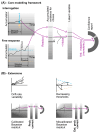
Figure 2. The Core Modelling Framework and Considered Extensions

Note. (A) All models considered are built from a core modeling framework in which observers track the total difference in evidence between alternatives (Bogacz et al., 2006). When the researcher sets the time of the response (interrogation condition), observers accumulate evidence until all information from the stimulus is processed (Bogacz et al., 2006). When observers set the time of response (free response condition), observers accumulate evidence until the accumulator reaches one of two decision thresholds (Ratcliff & McKoon, 2008). Evidence accumulation continues for a short time after a decision, as sensory and motor processing pipelines mean there will be additional information that did not contribute to the decision (Resulaj et al., 2009). (B) Model variants are constructed by adding combinations of possible extensions to the core model. Bayesian confidence—that is, the probability of being correct—is a function of time spent accumulating evidence and the amount of evidence accumulated (as represented by the shading). To be precise, in the Bayesian confidence models, the observer does not read out probability correct, but a monotonic function of this, as described in the main text. The function of time and evidence used by a miscalibrated Bayesian observer to estimate the probability of being correct differs from the function that would be used by a calibrated Bayesian observer. arb. = arbitrary; prob. = probability; est. = estimated. See the online article for the color version of this figure.

Figure 3. Participants’ Task Was to Determine Which Array Contained More Dots on Average

Note. The number of dots changed every 50 ms, resampled from two independent truncated normal distributions, one for each array. (“Free response”) In the free response condition, participants could respond when they liked. (“Interrogation”) In the interrogation condition participants had to respond within 1 s of a red cross appearing that marked the disappearance of the dot arrays. conf. = confidence; RT = response time. See the online article for the color version of this figure.

Figure 4. Duration of Sensory and Motor Processing Pipelines Was Estimated by Fitting a Step Function

Note. The step function was fitted to average evidence fluctuations in the frames running up to choices in the free response condition. Approach adapted from van den Berg, Anandalingam, et al. (2016). This figure shows an example fitted step function for one participant. See the online article for the color version of this figure.

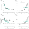
Figure 5. The Effect of Response Time on (A) Accuracy and (B) Confidence in the Main Study

Note. “Response” refers to the left vs. right choice. (B) Consistent with model predictions and with previous findings (Pleskac & Busemeyer, 2010), confidence decreased with response time in the free response condition, and the relationship between time and confidence was more negative in the free response condition than in the interrogation condition. The rationale for using binned confidence is explained in Models section. Similar patterns were obtained when plotting raw confidence scores against response time. Error bars represent ±1 SEM of the mean. Plotting details in Subsection “Plotting Procedure.” SEM = standard error of the mean. See the online article for the color version of this figure.

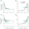
Figure 6. The Effect of Evidence Fluctuations on (A and B) Choices and (C and D) Confidence

Note. “Response” time refers to the left vs. right choice. Panels A and B plot the average evidence fluctuations in the direction of the choice made. This serves as a measure of the effect of evidence on the choice made (Experimental Method section; Resulaj et al., 2009). Panels C and D plot the rank correlation (Kendall’s τ) between evidence fluctuations and confidence. The shaded region in Panels B and D has a width equal to the median estimate, across participants, of the duration of sensory and motor processing pipelines. At time lags relative to response, all evidence appeared to be weighted equally in the interrogation condition (B). However, there was evidence that frames occurring at the onset of the stimulus were especially strong predictors of responses in both conditions (A). Looking at the free response condition data in Panel D, we see that evidence that was probably gathered after a decision (i.e., evidence probably in processing pipelines at the time of response) appears to have a greater effect on confidence, than the evidence that was probably processed prior to decisions. Error bars represent ±1 SEM of the mean. Plotting details in Subsection “Plotting Procedure.” SEM = standard error of the mean. See the online article for the color version of this figure.

Figure 7. The Effect of Predecision and Pipeline Evidence on Confidence in the Two Conditions

Note. The y-axis represents the values of coefficients produced by the ordinal regression onto confidence (Experimental Method section). We hypothesize that in the interrogation condition all evidence is processed prior to a decision, and therefore that there is no pipeline evidence. Nevertheless, as discussed in the main text, we artificially divide up the evidence presented, in the same manner as in the free condition, for the purpose of comparison. Unlike in other plots, error bars represent 95% confidence intervals. conf. = confidence. See the online article for the color version of this figure.

Figure 8. Model Comparison Results

Note. (A) Negative cross-validated log likelihood (−LLcv) relative to the model with the lowest mean −LLcv (Model DM with a mean −LLcv of 1.338) and (B) number of participants for which each model provided the best fit. A lower value of –LLcv in Panel A indicates better fit. Models in which confidence reflects a miscalibrated Bayesian readout fit best (Models M, VM, DM, VDM). Unlike in other plots, error bars represent 95% bootstrapped confidence intervals. V = drift-rate variability; D = decreasing thresholds; C = calibrated; M = miscalibrated.

Figure 9. (A-Av) Effect of Response Time and (B-Av) Average Evidence on Confidence in the Data (Error Bars) and in the Best Fitting Model, Model M (Shading)

Note. Model M accounted well for quantitative patterns in the effects of both response time and average evidence, and in differences between the two conditions. In Panel B average evidence is computed by summing, over all frames, the difference in dots presented in the two arrays, before taking the absolute value and dividing by the time the stimulus was presented for. In both A-Av and B-Av error bars and shading represent ±1 SEM. A-P10, A-P20, A-P30, B-P10, B-P20, B-P30 show corresponding data (circles) and model fits (lines) for three individual participants. Plotting details in Subsection “Plotting procedure.” Parameter values for key fitted models are given in Appendix F. Av = average; SEM = standard error of the mean; M = miscalibrated. See the online article for the color version of this figure.

Figure 10. Effect of Response Time and Evidence, Considered Simultaneously, in the (A-Av) Free Response and (B-Av) Interrogation Conditions

Note. Effect on confidence shown for the data (error bars), and in the best fitting model, Model M (shading). Except at the longest and shortest response times, Model M accounted well for the simultaneous effect of time and evidence in both conditions (A and B). Evidence is computed by summing, over all frames, the difference in dots presented in the two arrays, before taking the absolute value. We separated trials into tercile bins according to this value, separately for the two conditions and each participant. In both A-Av and B-Av, error bars and shading represent ±1 SEM. A-P10, A-P20, A-P30, B-P10, B-P20, B-P30 show corresponding data (circles) and model fits (lines) for three individual participants. Plotting details in Subsection “Plotting Procedure.” Av = average; SEM = standard error of the mean; M = miscalibrated. See the online article for the color version of this figure.

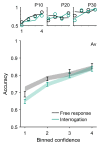
Figure 11. (Av) The Relationship Between Confidence and Accuracy in the Data (Error Bars) and in the Best Fitting Model, Model M (Shading)

Note. Generally, the model captured quantitative and qualitative patterns well. In Panel “Av” error bars and shading represent ±1 SEM. Panels “P10,” “P20,” and “P30” show corresponding data (circles) and model fits (lines) for three individual participants. Plotting details in subsection “Plotting Procedure.” Av = average; SEM = standard error of the mean; M = miscalibrated. See the online article for the color version of this figure.

Figure 12. Fit of the Best Model (Model M) to the Number of Confidence Reports in Each Confidence Bin in (A-Av) the Free Response Condition and in (B-Av) the Interrogation Condition

Note. The model fit is shown in shading and the data with error bars. The model captured quantitative and qualitative patterns very well. In both A-Av and B-Av error bars and shading represent ±1 SEM. A-P10, A-P20, A-P30, B-P10, B-P20, B-P30 show corresponding data (circles) and model fits (lines) for three individual participants. Plotting details in subsection “Plotting Procedure.” Av = average; SEM = standard error of the mean; M = miscalibrated. See the online article for the color version of this figure.

Figure 13. (A-Av and B-Av) The Effect of Evidence Fluctuations on Confidence in the Data (Error Bars) and in the Best Fitting Model, Model M (Shading)

Note. Effects shown (A) at times relative to trial onset and (B) at times relative to the response. To measure this effect, we computed the rank correlation (Kendall’s τ) between evidence fluctuations and confidence. The model accounted well for the effect of evidence at time lags relative to response (B-Av), in both conditions. However, the model failed to capture the strength of the effect of evidence presented at the onset of the stimulus (A-Av). In both A-Av and B-Av, error bars and shading represent ±1 SEM. A-P10, A-P20, A-P30, B-P10, B-P20, B-P30 show corresponding data (circles) and model fits (lines) for three individual participants. Plotting details in subsection “Plotting Procedure.” Av = average; SEM = standard error of the mean; M = miscalibrated. See the online article for the color version of this figure.

Figure 14. Model Fits for Two of the Losing Models

Note. Specifically, the effect of response time on confidence in the data (error bars), and in Models V and VC (shading). (A) Model V did not capture the strength of the effect of response time on confidence in the free response condition, (B) while Model VC slightly underestimated this effect. Error bars and shading represent ±1 SEM. Plotting details in subsection “Plotting Procedure.” Parameter values for key fitted models are given in Appendix F. SEM = standard error of the mean; V = drift-rate variability; C = calibrated. See the online article for the color version of this figure.

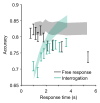
Figure 15. The Effect of Response Time on Accuracy in the Data (Error Bars) and in Simulations Using the Best Fitting Model for Confidence, Model M (Shading)

Note. The simulated behavior of the model was sensible, although there were clear differences to the data. The accuracy of model-simulated responses was too high at long response times. Error bars and shading represent ±1 SEM of the mean. Plotting details in subsection “Plotting Procedure.” SEM = standard error of the mean; M = miscalibrated. See the online article for the color version of this figure.

Figure 16. The Effect of Evidence Fluctuations on Choices, in the Data (Error Bars), and in Simulations From the Best Fitting Model for Confidence, Model M (Shading)

Note. Effects shown (A) at times relative to trial onset and (B) at times relative to the response. The model simulations were generally reasonable, and captured some key qualitative effects. The model simulations did not capture the strength of the effect of evidence presented at the onset of the stimulus (A). Error bars and shading represent ±1 SEM of the mean. Plotting details in subsection “Plotting Procedure.” SEM = standard error of the mean; M = miscalibrated. See the online article for the color version of this figure.

Figure 17. The Effect of Predecision and Pipeline Evidence on Confidence in the Two Conditions

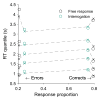
Note. Real data are shown with circles, while data simulated from the model are shown with crosses and connected by dashed lines. Following Ratcliff and McKoon (2008), for each participant and each unique combination of accuracy and condition (free response vs. interrogation), the 0.1, 0.3, 0.5, 0.7 and 0.9 quantiles of the response time distributions were calculated. The mean over participants is plotted on the y-axis. Data from a unique combination of accuracy and condition are plotted at the same x-value. This x-value represents the proportion of responses in that condition (free response or interrogation) that have the corresponding accuracy. Specifically, it is the mean of this value across participants. Note that this plotting procedure deviates from that described in subsection “Plotting Procedure.” Just as for other plots, the plot is based on trials in which a confidence report was obtained (meaning trials without a valid response in the interrogation condition are not included). RT = response time. M = miscalibrated. See the online article for the color version of this figure.

References

1. Acerbi L, Dokka K, Angelaki DE, Ma WJ. Bayesian comparison of explicit and implicit causal inference strategies in multisensory heading perception. PLOS Computational Biology. 2018;14(7):e1006110. doi: 10.1371/journal.pcbi.1006110. - DOI - PMC - PubMed
1. Adler WT, Ma WJ. Comparing bayesian and non-bayesian accounts of human confidence reports. PLOS Computational Biology. 2018;14(11):e1006572. doi: 10.1371/journal.pcbi.1006572. - DOI - PMC - PubMed
1. Ais J, Zylberberg A, Barttfeld P, Sigman M. Individual consistency in the accuracy and distribution of confidence judgments. Cognition. 2016;146:377–386. - PubMed
1. Aitchison L, Bang D, Bahrami B, Latham PE. Doubly bayesian analysis of confidence in perceptual decision-making. PLOS Computational Biology. 2015;11(10):e1004519. doi: 10.1371/journal.pcbi.1004519. - DOI - PMC - PubMed
1. Audley RJ. A stochastic model for individual choice behavior. Psychological Review. 1960;67(1):1–15. - PubMed